Optimization of automatic control system parameters
Laboratory work No.7 on the course "Control in technical systems"
Purpose of the work
- Familiarization with the optimization procedures in SimInTech on the example of the synthesis of the optimal integral controller
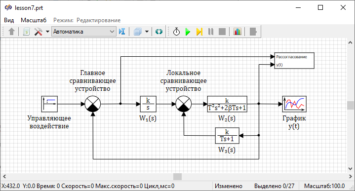
Formulation of tasks for parametric optimization of ACS
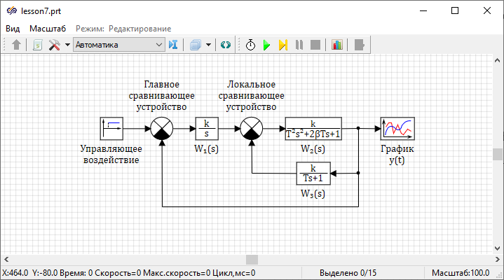
- "Gain factor" = "1"
- "Time constant" = "1"
- "Damping factor" = "0.5"
- "Gain factor" = "0.6"
- "Time constant" = "5"
- when applying a step disturbance, there is no overshoot
- setting time does not exceed 20 s
When performing laboratory work No.1, the direct modeling method was used, which made it possible to determine the value of the controller gain equal to "0.35" in just three attempts, in which the transient in the ACS simultaneously satisfied both of the above limitations.
If there is no recommendations for varying speed gain values, the search for the optimal value could be difficult. With an increase in the number of variable parameters, the search strategy by the selection method becomes not obvious.
SimInTech implements a block Optimizer, which allows to perform an automated search for such values of the variable parameters of the ACS, in which the dynamic characteristics of the ACS (and the transient process, in particular) meet the optimality criteria.
Sequence of actions for optimization
- Set variable parameters as global variables (more precisely, the project signal) using the appropriate interface procedures
- Form local optimization criteria that are necessary to solve the main optimization problem
- Put the block on the diagram Optimizer and enter the required data in its settings, including:
- names of variable parameters, their range limits and simulation error
- names of local criteria and permissible limits of their values
- calculation method of optimization and its settings
- Start simulation
Setting the variable parameter as a global project signal
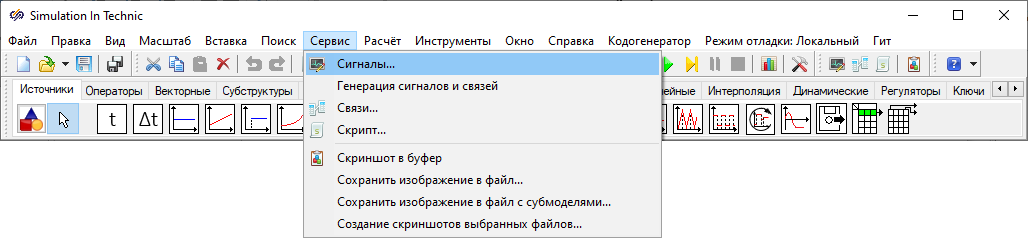
The project signal list allows you to create a list of variables that are used in the simulation process and provide access to these variables by their name.
In the window List of project signals click button Add signal to add a new signal with the possibility of changing its parameters.
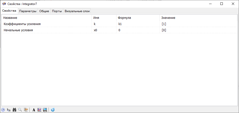
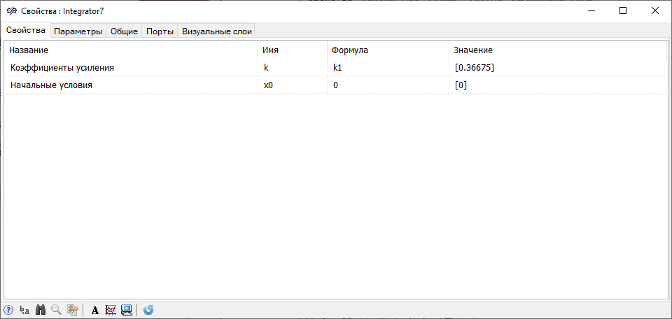
- “k1" – gain factor - parameter that is optimized in the task
- "tpp" – setting time
- "dy" – overshoot value
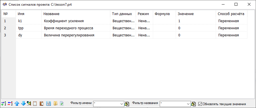
The variables of this list can be used as properties of the blocks of the simulation diagram.
Simulation of local optimization criteria
To simulate the parameters of the transient process, a submodel is used, in which a computational scheme will be created.
Put the block on the diagram Submodel from tab Substructures and enter the submodel. To the workspace of the block Submodel place two blocks Input port. It is recommended to place them on the left side one under the other, then their order will correspond to the order of the inputs of the block to schematic of the upper level.
- 1 block Absolute value from tab
- 1 block Clock from tab Sources
- 1 block Key-3 from tab Keys
- 1 block Delay on the integration step from tab Nonlinear
- 1 block Lower or upper limit from tab Nonlinear
- 2 blocks Output port from tab Substructures
- 2 blocks Recording to the list of signals from tab Signals
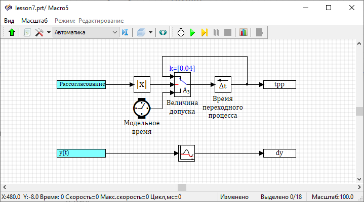
- In the properties of the block labeled "Tolerance value" (Key-3) in the "Setpoint values" line, enter a value equal to "0.04", which corresponds to a 5% tolerance for the future steady state value
- In the block properties Lower or upper limitset "Operation type" – "Maximum". This block will record the maximum value of the value received from the input port in the signal list
- Double-click on the blocks Input port to open window Submodel port and in the "Submodel port names" field, set the port names "Error" and "y(t)" in accordance with Figure (Figure 6)
- In the block properties Recording to the list of signals set the "Signal names"property to "tpp" and "dy" according to Figure (Figure 6)
- To the middle (logical) input port of the block Key-3 (tolerance value), the absolute value of the error is supplied
- If this signal is greater than the setpoint (5% of 0.8), then to the block output Key-3a signal is transmitted from the third (lower) input port, i.e. the current model time
- If the control signal (at the middle input port) is less than the setpoint, then to the block outputKey-3 a signal is transmitted from the first (upper) input port, i.e. the same signal, but delayed by one integration step
- The delay on the integration step is carried out by a block labeled "Setting time" (block Delay on the integration step from tabNonlinear)
Thus, after the simulation is completed, the variables "tpp" and "dy" will contain the value of the setting time and the maximum value of the output from the block with the label "W2(s)".
Exit the submodel workspace by double-clicking on the free space of the project window or by clicking the button Back from submodel.
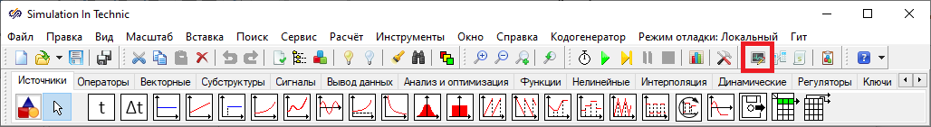
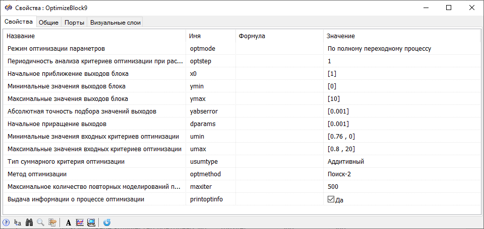
Setting up the "Optimizer" block
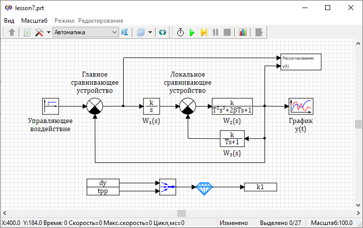
- 2 blocks Reading from signal list from tab Signals
- 1 block Recording to the list of signals from tab Signals
- 1 block Multiplexer from tab Vector
- 1 block Optimizer from tab Analysis and optimization
Configure the blocks Reading from signal list and Recording to the list of signals according to Figure (Figure 8).
Description of the schematic operation: two signals, the maximum value – "dy", and the setting time – "tpp", calculated in the block Submodel, are packed in a vector and transmitted to the block Optimizer, this block calculates the value transmitted to the signal "k1", which, in turn, determines the property "Gain factor" in the block with the label "W1(s)", and must provide the specified characteristic of the transient process.
As optimization parameters, we use the setting time and the maximum value during the transient process, respectively, optimization should be calculated for the entire transient process.
Block Optimizer can simulate optimal values also during the transient, but for this it is necessary to use the optimization criteria calculated at each time point.
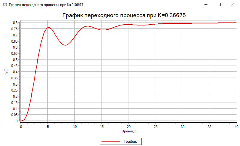
Simulation of the optimal controller
By clicking the button Start simulation is started in the main window. It should be noted that with the added optimization block in the "Over the full transient" mode, the model in SimInTech is calculated not once in dynamics, but several times until the optimal result is obtained. In this case, information about the optimized parameter and the reached optimization criteria appears in the message window, at the bottom of the schematic window.
Conclusion
The demonstration and introductory task is completed. The project must be saved.