Development of a non-linear ACS of a nuclear reactor
Laboratory work No.5 on the course "Control in technical systems"
Introduction
A typical automatic control system of a nuclear reactor is a high-dimensional control system. A detailed study of the dynamical properties of such an ACS using numerical modeling methods is a complex scientific and technical problem, since there are technical devices in the reactor plant (RP) that use information from most fundamental and applied sciences to describe dynamical processes.
Until the early 90s of the last century, specialized dynamical programs (applied to a specific plant) were developed to study non-stationary processes in complex controlled technical systems. The use of such programs to study non-stationary processes in the case of, for example, a significant modernization of the same plant required a serious redesign of the simulation program at the source code level (mathematical models, algorithms, etc.), which only the programmers who created this program were really able to perform.
Significant progress made in the last decade in the hardware and software capabilities of modern computing has created the necessary basis for the development of fundamentally new intelligent CAE tools, for example, object-oriented software environments for the study of non-stationary processes in complex dynamical systems.
Currently, a number of modern software packages have been created in the Russian Federation for the study of non-stationary processes in reactor plants.
- firstly, each of them can be recommended for use in the design development of new reactor plants of a similar type only
- secondly, none of these software packages is suitable for use in the educational process of higher education due to the lack of appropriate methodological content
The software of intelligent CAE also includes SimInTech, one of the main advantages of which is invariance to the subject area of the object or physical phenomenon under study. This allows SimInTech to perform a numerical study of working processes in almost any complex technical systems: in electromechanical, thermal-hydraulic, pneumatic and hydraulic systems and in a number of other combined dynamical systems, including reactor systems.
SimInTech uses simpler but faster mathematical models than the aforementioned industry-specific software tools to describe the dynamics of neutronic and thermal-hydraulic processes in nuclear reactors. Also, modularity and integration with many specialized calculation codes allows using SimInTech as an integrating platform when creating complex complex models of dynamics (simulators for NPP operators, operators of main powerplants of of mobile facilities, virtual power units, and so on).
The software and hardware capabilities of SimInTech qualitatively exceed the capabilities of Russian-developed industry software in the tasks of developing mathematical models of automatic and logical control systems, protection and interlocking systems in relation to the design justification of PCS for NPP units with pressurized water reactors (VVER-type reactors), high power channel-type reactors (RBMK-type reactors), fast reactors of various types and others.
An equally important advantage of SimInTech is its adaptability: from the simplest dynamic tasks for educational purposes to real industry developments, including those in the export version.
The presence of detailed educational and methodological support in SimInTech allows it to be used in the educational process of higher education in many engineering specialties.
In previous laboratory work, we mastered some of the methods of work in SimInTech. In this laboratory work, it is possible to master a number of new methods of work, as well as to perform an independent numerical study of the dynamic characteristics of a simplified mathematical model of a nonlinear ACS of a nuclear reactor with a relay-type controller.
Purpose of the work
- Familiarization with the description of mathematical models of neutron kinetic processes from the library Neutron kineticsinclusive of:
- comparative analysis of the frequency and transient characteristics of the kinetics of a nuclear reactor using a single-group and classical (6-group) description of the precursor nuclei of delayed neutrons
- comparison of the transient characteristics of the kinetics of a nuclear reactor without taking into account and taking into account the decay heat
- Self-study of non-stationary processes in a nonlinear ACS of a nuclear reactor (NR ACS) with a relay controller, including:
- formation of a mathematical model of NR ACS with a relay controller
- simulating of transients when varying the parameters of NR ACS
Mathematical models of neutron kinetics
LibraryNeutron kinetics SimInTech includes three blocks, two of which describe the neutron kinetic processes in a nuclear reactor in a single-speed point approximation, and the third describes the dynamics of the decay heat, taking into account the past of the reactor.
The first two blocks make it possible to describe the kinetics of precursor nuclei of delayed neutrons from single-group to n-group approximations. Mathematical models of these blocks are obtained on the basis of the known equations of kinetics of a point nuclear reactor in a single-speed approximation (i.e. the process of fission of nuclei is carried out by neutrons of the same energy group – either only thermal neutrons or only fast neutrons):
- N(t) – reactor power
- r(t) – reactivity
- βeff – effective fraction of delayed neutrons
- l – prompt neutron lifetime
- Ci(t) – concentration of precursor nuclei of delayed neutrons of the i-th group
- λi – decay constant of the precursor nuclei of the i-th group
- βi – fraction of delayed neutrons of the i-th group
- S(t) – intensity of the external neutron source
First block Point kineticscorresponds to a constant (over time) intensity of the external neutron source. Input is a reactivity differential
and output – either a dimensionless deviation of power
or normalized power
After the transformations, the initial system of equations takes the form:
- – normalized deviation of the concentration of precursor nuclei of delayed neutrons of the i-th group
- – absolute (modulus) subcriticality of a nuclear reactor
- – fractional change of reactivity, in fractions of βeff
- – relative fraction of delayed neutrons of the i-th group
At t = 0, the reactor is stationary, so
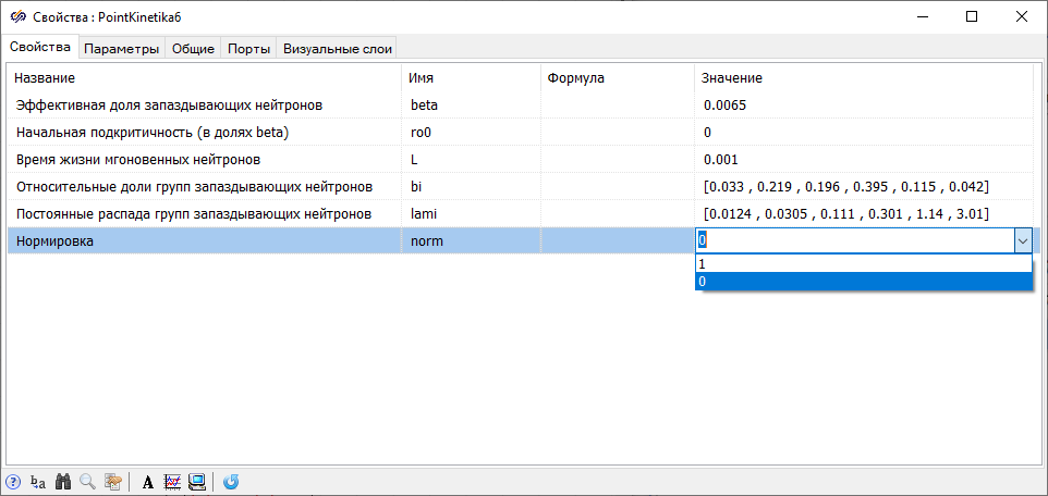
The value of the prompt neutron lifetime approximately corresponds to the lifetime in the high power channel-type reactor (RBMK-type reactor).
The values in the last row of the "Normalization" properties correspond to the following types of the output signal of the block: 1 – normalized power
and 0 – dimensionless power deviation
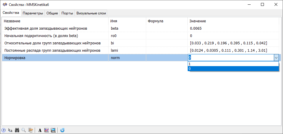
The second typical block Point kinetics (prompt jump model) corresponds to the prompt jump model. The input is a reactivity increment:
and the output – either the normalized power:
and either a dimensionless power deviation:
The neutron kinetics equations after the transformations of the initial system of equations take the form:
where
and the rest of the designations coincide with the system for the block with the classical model of neutron kinetics. Obviously, if at t ≤ 0 the neutron power is constant, then the initial conditions for c~i(0) are 1.0.
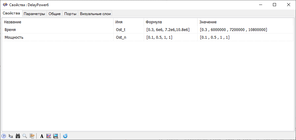
The figure shows the properties window of this block (Figure 2), where, by default, β*i and λi correspond to the data for the 235U fuel, and the values of the "Normalization" property have the same meaning as in the properties window of the block Point kinetics.
where N(0) – stationary state power value at t = 0.
The third typical block Decay heat (according to ANSI) from tab Neutron kinetics makes it possible to take into account the additional contribution of the decay heat of fission products to the reactor thermal power, which is especially important in case of sharp decreases in neutron power. The input signal to the block is the relative neutron power (normalized to the nominal neutron power), and the output signal from the block is the relative reactor thermal power (normalized to the nominal neutron power), determined by the expression:
where – reactor thermal power and decay heat, normalized to the nominal neutron power, respectively.
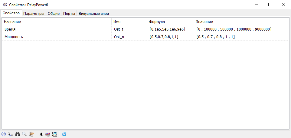
- at 0 s ≤ t ≤ 105 s, the relative neutron power of the reactor (normalized to the nominal neutron power) was 0.5
- at 1×10⁵ s < t ≤ 5 ×10⁵ s n~ = 0.7
- at 5 ×10⁵ s < t ≤ 1 ×10⁶ s n~ = 0.8
- at 1×10⁶ s < t ≤ 9×10⁶ s n~ = 1.0
Comparison of classical and single-group models of neutron kinetics
When performing previous laboratory work and self-guided tasks on the TSC course, the simplest mathematical models of neutron-kinetic processes in a nuclear reactor were used, namely a point model with one effective group of delayed neutrons.
When considering long transients, the value of the effective decay constant λ of precursor nuclei of delayed neutrons in a single-group model is recommended to be obtained by averaging the "lifetime" of groups of delayed neutrons by the ratio:
which gives a value of λ = 0.0767 s-1 (in some textbooks, λ = 0.072 s-1 is given).
When considering short transients (for example, the initial stage of the development of a transient with a significant reactivity jump), the value of the effective decay constant λ of the precursor nuclei of delayed neutrons in a single-group model can be obtained from the ratio:
which gives a value of λ = 0.405 s-1.
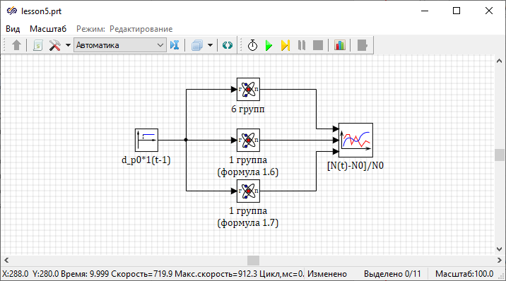
d_p0 is set by the parameter k (in fractions of βeff). The global constants Lam and Lam_1 are effective decay constants calculated from the ratios, respectively.{Setting the reactivity exposure}
b_eff=0.0065; k=0.01; d_p0=k*b_eff;
{Setting the relative fractions of groups of delayed neutrons}
b1=0.033; b2=0.219; b3=0.196; b4=0.395; b5=0.115; b6=0.042;
{Setting the decay constants of precursor nuclei of delayed neutrons}
lam1=0.0124; lam2=0.0305; lam3=0.111; lam4=0.301; lam5=1.14; lam6=3.01;
{Calculation of the decay constants of precursor nuclei}
Lam=1/((b1/lam1)+(b2/lam2)+(b3/1am3)+(b4/lam4)+(b5/lam5)+(b6/lam6));
Lam_1=(b1*lam1)+(b2*lam2)+(b3*lam3)+(b4*lam4)+(b5*lam5)+(b6*1am6); Open the table with calculated data by clicking on the button Calculate all. Ensure that the calculated values of the effective decay constants of the precursor nuclei for short and long transients match the above values.
Close the project script and set the properties of the block diagram blocks. In the block with the label "6 groups" (describing the six group model of neutron kinetics), no change in properties is required.
- "Relative fractions of delayed neutron groups" equal to "1"
- "Decay constants of groups of delayed neutrons" in the "Formula" field are equal to "Lam" and "Lam_1", respectively.
Determine yourself the properties of other blocks.
- "End calculation time" = "1000"
- "Minimum step" = "1e-10"
- "Maximum step" = "0.1"
- "Integration method" = "Adaptive 1"
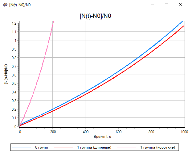
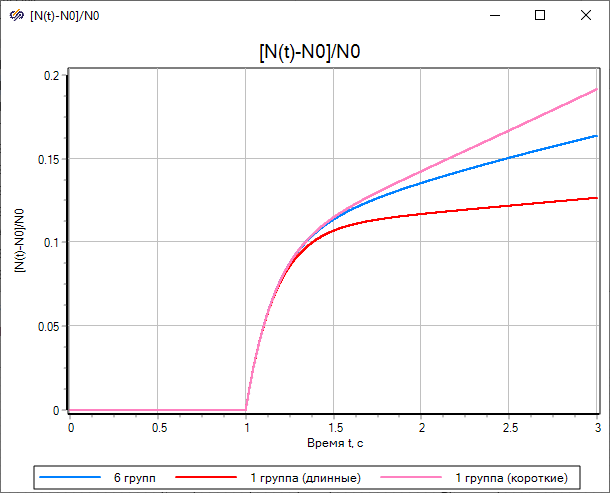
The blue line shows the transient plot for the classical neutron kinetics model, the red line for the single-group model with the effective decay constant "Lam" calculated by the ratio, and the pink line for the single-group model with the effective decay constant "Lam_1" calculated by the ratio.
The result of the simulation shows that with the effective decay constant "Lam", the one-group model of kinetics only approximately corresponds to the classical model of kinetics, and with the effective decay constant "Lam_1" – the difference is huge (at t = 1000s about 40 times).
- "End calculation time" = "3"
- "Minimum step" = "1e-10"
- "Maximum step" = "0.001"
- "Integration method" = "Adaptive 1"
Simulate the frequency characteristics for the classical and one-group models of neutron kinetics (for both options of λ calculation).
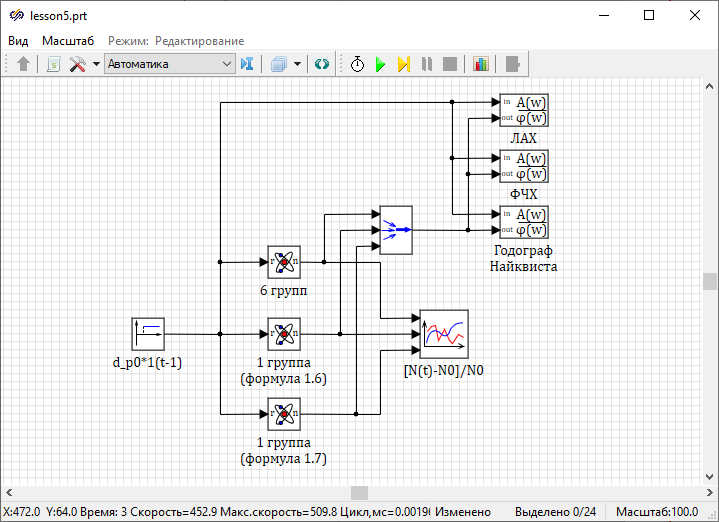
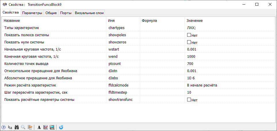
Similarly for the block labeled "Magnitude plot", set the properties of the block labeled "Phase plot" and the block labeled "Nyquist plot" by changing the value of the parameter "Characteristic type" to "Phase plot" and "Nyquist plot", respectively.
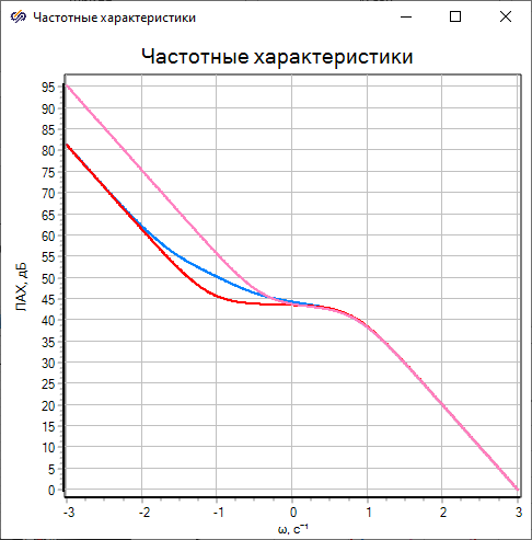
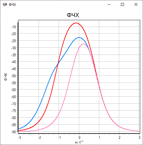
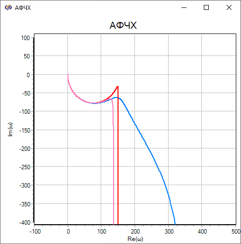
The analysis of the plots (Figure 9 and Figure 10) confirms the previously noted coincidence of frequency properties for all three variants of the mathematical model of neutron kinetics at high frequencies and, vice versa, a noticeable difference in the magnitude plot and the phase plot at low frequencies.
In Figure (Figure 11), the blue double-thickness line shows the plot for the classical neutron kinetics model, the red line for the single-group model with the effective decay constant Lam calculated by the ratio, and the purple line for the single-group model with the effective decay constant Lam_1 calculated by the ratio. Analysis of the data shows that in the high-frequency range all three loci almost coincide, and in the low-frequency range there is a noticeable difference.
- A single-group model of the neutron kinetics of a nuclear reactor without a controller or negative reactivity effects for any method of calculating the effective decay constant cannot provide a correct quantitative description of the transients
- According to the frequency properties of the two options of the one-group model, the classical model of neutron kinetics is much closer to the option with the effective decay constant calculated by the ratio
Thus, when simulating the dynamics of NR ACS under the control signal, it is preferable to use an option with the value of the effective decay constant obtained by the ratio, and if the dynamics of NR ACS is simulated with a significant perturbing reactivity exposure, it is preferable to use an option with the effective decay constant calculated by the ratio.
The role of decay heat in the dynamics of a nuclear reactor
If the nuclear reactor operates in the vicinity of the nominal mode, then only the neutron kinetics equations can be used to calculate its power (neutron, Nn, and thermal, NT), since in this case the values of the relative neutron power (normalized to the nominal neutron power, Nnnom) and the relative reactor thermal power (normalized to the nominal reactor thermal power, NTnom) are approximately equal to:
If the reactor neutron power has changed dramatically, then the contribution of decay heat should be taken into account when calculating thermal power.
Perform a quantitative assessment of the validity of the above mentioned fact by direct simulation of the following possible emergency situation: free fall of one of the emergency protection rods having a reactivity worth equal to 1.0×βeff.
At the time of the emergency, the nuclear reactor had a operating cycle length of three thousand hours, with the first thousand hours of the reactor operating at a 10% percent power level, then a thousand hours at a 50% power level, and finally the last thousand hours at the nominal power level.
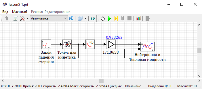
The formed example shows the principle of operation of the rod fall, where the rod is above the core for ten seconds, and then for one second the rod falls into the core, while negative reactivity (1.0×βeff) is introduced into the reactor according to the linear law of time. In the properties of the block labeled "Rod fall law", set the property "Time" equal to "[[10.1, 11.1]]", the property "Value of the function" equal to "[[0, -0.0065]]".
Block Gain implements normalization of the reactor thermal power, and the label of the block "1/1.0658” indicates that at the time of the emergency, the additional contribution to the decay heat thermal power is 6.58%. After setting the parameters of all blocks in the block diagram, it is necessary to check the value of the contribution. To proceed this, you need to initialize the block diagram and then use the "hotline".
- "End calculation time" = "200"
- "Minimum step" = "1e-12"
- "Maximum step" = "0.1"
- "Integration method" = "Adaptive 1"
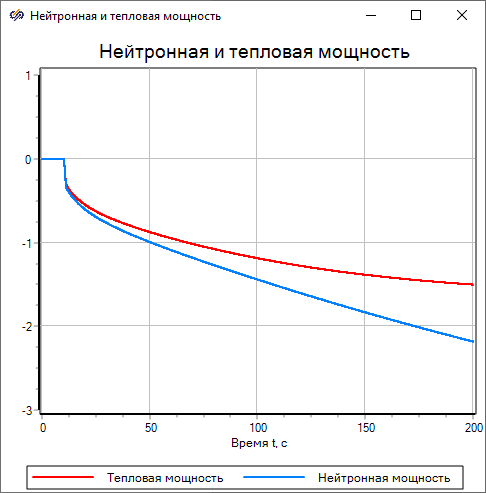
The solid red line of double thickness represents the behavior of the relative thermal power, and the blue line represents the behavior of the relative neutron power. The data in the figure show that at approximately 170 seconds, the relative neutron power reached 1% of the nominal value, while the relative thermal power reached a value of more than 3% (Figure 14).
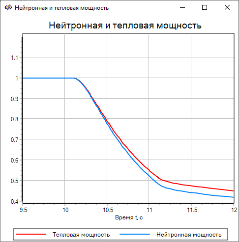
The data in the figure show that when the neutron power is reduced to approximately 70% of the nominal value, the plots of the relative neutron power and the relative thermal power practically coincide, and when the power is further reduced, a noticeable difference appears (Figure 15).
Thus, with a sharp decrease in the neutron power of a nuclear reactor, it is necessary to take into account the contribution of decay heat into the thermal power.
Block diagram of nuclear reactor ACS
As part of this laboratory work, it is worth considering a simplified nuclear reactor ACS, the block diagram of which is shown in the figure and corresponds to a non-linear relay-type ACS (Figure 16).
Most of the blocks in the block diagram are located in the libraries of the groupAutomatics. Block Point kinetics located in the library Neutron kinetics.
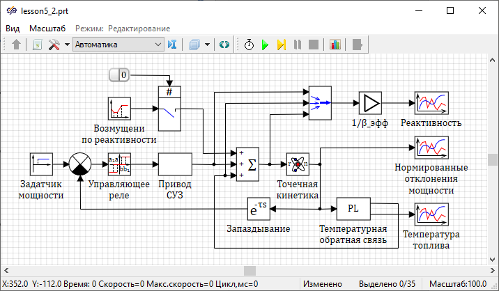
In this NR ACS, the error signal is transmitted to the block with the label "Control relay", which, when the setpoints are exceeded, generates a control signal to move the control rod at a constant speed up or down. Such relay control significantly reduces wear of the control rod drive mechanism compared to the principle of continuous monitoring of the NR power.
The reactivities of the control rod, the temperature effect and the NR itself are "compressed" by means of a multiplexer into a vector signal, then vectorly normalized to the effective fraction of delayed neutrons and displayed on the corresponding plot.
A block is included in the main feedback circuit Ideal transport delay, which simulates the time delay connected with processing the readings of the neutron flux detectors.
In this laboratory work, the input of reactivity perturbations is performed using a block Piecewise linear from tab Sources.
The block labeled "Master comparator" operates in subtraction mode.
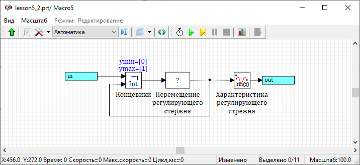
- a block labeled "Travel of the control rod" simulates the movement of the control rod
- block Integrator key from tabKeys simulates reaching the upper or lower limit switches
- block Sinusoidal function sets the value of the reactivity that the rod introduced into the reactor
- the blocks Input port and Output port provide data exchange with other blocks in the system
Description of mathematical models of reactor ACS blocks
Since the dynamics of ACS will be analyzed mainly in normalized deviations, it is more expedient to use the classical model of point kinetics with six groups of delayed neutrons to describe neutron kinetics. It is assumed that at t ≤ 0 the reactor is in a stationary state, so at t = 0 at the block outputPoint kinetics n~(0) = 0.
The block labeled "Master Comparator" implements normal subtraction, and the block Summator implements algebraic addition of input signals.
In the block labeled "Control relay", the amplitude of the function values is "1", and the values of the other properties will be set by the instructor.
The dynamics of the block labeled "Temperature feedback" is described by the following equations:
- N(t) – reactor power (absolute)
- T(t) – fuel temperature
- Tw – coolant temperature (in this work it is considered constant)
- T0 – fuel temperature in the stationary state
- K – coefficient proportional to the heat exchange between the nuclear fuel and the coolant
- c, g, V – specific heat capacity, density and volume of fuel, respectively
The block labeled "Travel of the control rod" is described by the following dynamic equation:
- x(t) – relative position of the lower end of the control rod (x = 0 – the rod is completely immersed in the core, x = 1 – the rod is completely removed from the core):
- kdr, tdr – relative speed of the control rod and the time constant, respectively
At t = 0, the control rod is stationary and half-immersed in the core, i.e. x(0) = 0.5.
The block labeled "Control rod characteristic" is described by the following inertia-free nonlinear equation:
Setting ACS parameters through the mechanism of global constants and variables
Some parameters of mathematical models of block dynamics must be set in the windowPage script.
The greatest effect from using global constants and variables will be achieved in cases where the same parameter is used in the properties of a large number of blocks in a block diagram. In this case, when changing the value of this property, you can only adjust its value in the project script, rather than adjusting its value in all blocks where it is used.
initialization
    c_t=300;           //Heat capacity of fuel, J/kg*K
    gam_t=1e4;         //Density of fuel, kg/m^3
    v_t=0.2;         //Volume of fuel,
    alfa=6.5e-5;      //Temperature coefficient of reactivity, 1/К
    T_o=700;           //Fuel temperature in the stationary state,
    T_w=500;           //Coolant temperature in the stationary state, K
    beff=6.5e-3;      //Effective fraction of delayed neutrons
    pmax=0.4*beff;   //Reactivity worth of the control rod
end;
In the block properties Point kinetics In the "Formula" field of the "Effective fraction of delayed neutrons" property, set the value to "beff". In the properties of the block labeled "1/β_eff", in the "Formula" field of the "Gain factor" property, set the value to "1/beff". In the submodel labeled "Control rod drive" in the block Sinusoidal function set the property "Amplitude" in formula a*sin(w*x(t)+f)" equal to "pmax".
Forming the dynamical model of the block "Programming language" labeled "Temperature feedback"
input u; {Description of the input signal name and dimension}

init T=700; {Setting the initial value for dynamic variable}

No=1e7;
n=u;
N=No*(1+n);
K=No/(T_o-T_w);
T'=(N-K*(T-T_w))/(c_t*gam_t*v_t);
po_oc=-alfa*(T-T_o);

output po_oc, T; {Description of names and dimensions of the output signals} input u;) assigns the input a unique name "u".The init operator describes the initial conditions for dynamic variables describing the initial conditions for dynamic variables that will be written as ordinary differential equations in Cauchy form.
In this example, the second executable line (init T=700;) sets the initial value for the only dynamic variable (fuel temperature at stationary state).
The differential equation for fuel temperature is written in the sixth executable line, where the apostrophe symbol denotes the derivative with respect to time, and the thermophysical properties of the fuel and the temperature of the coolant in the stationary state are transferred to the block Programming language by means of global constants and variables.
The next to last executable line describes the reactivity effect by fuel temperature.
In this example, the last line (output po_oc, T;) describes two output signals, "po_oc" and "T", without specifying the dimensions of the output signals in square brackets.
Block Programming language in the project window will have one input and two outputs. The first output port "T" will be at the top right, and the second output port "po_os" will be at the bottom right.
Complete the block diagram in the project window by connecting all blocks with signal lines. The block diagram of the ACS should look similar to (Figure 16).
Independent work
Table (Table 1) shows the initial data on the parameters of the NR ACS elements to be studied.
| No. | ACS element | Parameters of ACS elements | Option number | ||
|---|---|---|---|---|---|
| 1 | 2 | 3 | |||
| 1 | Power demand | Time, s | 10 | 10 | 10 |
| Y0 | 0 | 0 | 0 | ||
| Y1 | 0.1 | 0.1 | 0.1 | ||
| 2 | Control rod drive | r*rod/ βeff | 0.6 | 0.6 | 0.6 |
| tdrive,s | 0.2 | 0.25 | 0.2 | ||
| Тfull stroke, s | 5...50 | 5...50 | 5...50 | ||
| 3 | Control relay | B | 0.02...0.005 | 0.02...0.005 | 0.02...0.005 |
| M | 0.4 | 0.6 | 0.8 | ||
| 4 | Nuclear reactor | V, m3 | 0.1 | 0.2 | 0.4 |
| gfuel, kg/m3 | 10000 | 9000 | 8000 | ||
| Сfuel, J/kg×К | 300 | 350 | 400 | ||
| l×103, s | 1 | 0.1 | 0.05 | ||
| βeff×103 | 6 | 6.5 | 7 | ||
| N₀, MW | 10 | 20 | 50 | ||
| 5 | Temperature feedback | T₀, K | 700 | 750 | 800 |
| Tw, K | 500 | 550 | 550 | ||
| a×104, 1/K | 0.7...1.5 | 0.7...1.5 | 0.7...1.5 | ||
| 6 | Disturbance | Δtdist | 2...20 | 2...20 | 2...20 |
| Δrdist/ βeff | 0.1...0.3 | 0.1...0.3 | 0.1...0.3 | ||
| 7 | Measurement channel delay | tmdelay, s | 0.2...1 | 0.2...1 | 0.2...1 |
In the submodel labeled "Control rod drive mechanism",” the Tfull stroke property indicates the time required for the control rod drive mechanism to travel its whole length (height) of the core. This property must be used to determine the drive speed gain coefficient. In Figure (Figure 17), the transfer function of the block labeled "Travel of the control rod" is unknown. This block must be determined based on the dynamic equations.
In the block labeled "Disturbance by reactivity" the parameter Δtdist specifies the time during which the disturbance value changes linearly from zero to Δrdist.
The data in the table (Table 1) of the type "5...50" implies that the study should be performed while varying the corresponding parameter within the specified range (the range implies the use of 4-5 equidistant points).
In a self-guided part of the laboratory work, the following steps should be performed:
- Using the block palette, editing procedures, and service procedures, form a block diagram with the necessary blocks and make its appearance similar to the figures (Figure 16, Figure 17)
- Using The Page script and the block property windows set their values for simulation of the diagram
- Using the block Programming language, form the mathematical model of the block labeled "Temperature feedback"
- With the initial values of the block diagram parameters (a = 7·10-5 1/K, tdelay = 0.2 s, Tfull stroke = 20 s, b = 0.02), perform simulation ("End calculation time" - "100") of the process of transferring the reactor to increased (+10%) and reduced (-10%) power levels while varying the drive gain (while varying Tfull stroke).
- Restore the parameters of the block diagram to their initial state and simulate the process of transferring the reactor to increased (+10%) and reduced (-10%) power levels while varying the measurement channel delay (when varying tdelay)
- Restore the parameters of the block diagram to their initial state and simulate the process of transferring the reactor to an increased (+10%) power level while varying the temperature feedback coefficient (when varying a)
- Restore the parameters of the block diagram to their initial state and simulate the process of transferring the reactor to an increased (+10%) power level while varying the deadband width in the control relay (when varying β)
- Restore the parameters of the block diagram to their initial state and simulate (simulation time up to 20 s) the transient when applying a disturbance Δrdist= 0.1⋅βeff and varying the disturbance input rate by reactivity (when varying Δtdist)
- Restore the parameters of the block diagram to their initial state and simulate the transient when applying a disturbance Δtdist = 5 s and varying the disturbance value by reactivity (when varying Δrdist)