Development of a control system based on fuzzy logic with code generation in DLL
Laboratory work No.8 on the course "Control in technical systems"
Introduction
SimInTech is a tool for creating mathematical models of any systems, the description of which can be presented in the form of systems of algebraic and ordinary differential equations.
To simplify the process of modeling complex branched systems, SimInTech allows you to use graphical animation of blocks, which change their graphical display depending on the calculated parameters.
To speed up simulation and check the performance of the developed algorithms as embedded control algorithms, SimInTech allows you to convert computational schematics of control algorithm models into dynamic-link libraries (DLLs) using automatic generation of C code and use these DLL instead of the original schematics of control algorithm models.
At the first stage of this laboratory work a study of the work of animated blocks will be carried out using the example of library blocks Fuzzy logic. At the second stage, a model of a control system based on fuzzy logic will be developed to maintain the specified water level in a leaky tank. At the third stage, the fuzzy controller will be converted to the form of a dynamic-link library (DLL) using automatic code generation.
Purpose of the work
- Explore work of animated blocks using the example of the blocks of the libraryFuzzy logic
- Acquire primary skills to develop a control system model based on fuzzy logic
- Learn how the SimInTech code generator works
Tasks of the work
- Study the principle of constructing the Mamdani fuzzy inference system
- Develop a model for studying the operation of animated blocks based on fuzzy logic
- Study operation of the animated blocks
- Develop a model of the leaky tank control system:
- develop a model of a leaky tank
- develop a valve model
- develop a controller model based on fuzzy logic
- Draw the plots showing the dependence of the target and current water levels in the tank over time, and a plot showing the outlet flow rate dependence over time.
- Compare the plots of the target and current water level in the tank
- Convert a fuzzy controller to a dynamic DLL using a code generator
- Compare the operation of the system model with the converted fuzzy controller with the operation of the initial system model
Basic theoretical information
In the classical theory of automatic control, the control signal on the system is calculated depending on the controlled value expressed in numerical form, and the control system converts the input parameters into control signals by transfer functions.
- IF "input parameter" = "A", THEN "control signal" = "B"
- IF "input parameter 1" = "A1" AND/OR "input parameter 2" = "A2", then "control signal" = "B"
- IF "water temperature" = "hot", THEN "command" = "open cold water valve"
- IF "water temperature" = "cold", THEN "command" = "open hot water valve"
- IF "water temperature" = "cold" AND "hot water valve" = "fully opened", then "command" = "close cold water valve"
- IF "water temperature" = "hot" AND "cold water valve" = "fully opened", then "command" = "close hot water valve"
- IF "level" = "high", THEN "valve control signal" = "close fast"
- IF "level" = "normal", THEN "valve control signal" = "do not change"
- IF "level" = "low", THEN "valve control signal" = "open fast"
- IF "level" = "normal" AND "rate of level change" = "decreases", THEN "valve control signal" = "open slowly"
- IF "level" = "normal" AND "rate of level change" = "increasing" THEN "valve control signal" = "close slowly"
In these examples, the control signal is determined not in numerical form depending on the numerical value of the water temperature or the value of the water level in the tank, but in the form of a logical analysis of the statements.
To build control algorithms based on fuzzy logic, the data transmitted to the control unit based on fuzzy logic must be converted. To do this, it is necessary to convert the input and output parameters linguistic variables. Each linguistic variable is characterized by a set of terms.
- the linguistic variable "water temperature" may have the following terms: "cold", "normal", "hot"
- linguistic variable "level" – terms: "low", "normal", "high"
- linguistic variable "valve control signal" – "open fast", "open slowly", "do not change", "close fast", "close slowly"
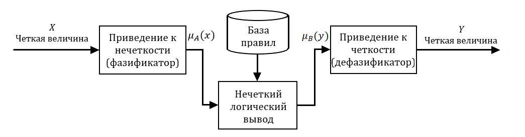
Each term is defined by its membership function μi(x), which can take values from 0 to 1. For each value of the input variable x, the values of μi(x) for each term are calculated. This procedure of converting an crisp input of input quantities into a fuzzy set, determined using the values of the membership functions μi(x), is called fuzzification.
After fuzzification, a set of rules is applied. The result of applying the rule is a quantity called the truth degree, which takes a value from 0 to 1. For example, let's say for the following rule:
IF "level" = "low", THEN "valve control signal" = "open fast",
the input value indicating the level, h, is given in meters. If the value of the level is low (μlow(h) = 1, where μlow(h) is the membership function for the term "low"), or the level is not low (μlow(h) = 0), then the truth degree of the rule takes the value of 1 or 0, similar to classical logic. Fuzzy logic applies if the membership function takes a value from 0 to 1, that is, if 0 < μlow(h) < 1. So, μlow(h) = 0.5 means that the level is not low and not high, respectively, the valve opening speed should be between fast and slow. In this rule, the truth degree of the statement "open fast" is 0.5.
Similarly, the truth degree for each rule is calculated. If in the condition rule. This procedure is called aggregation. The calculated truth value for all conditions of each rule is applied to the statements of each rule. This process is called activation. Aggregation and activation form a fuzzy inference.
- μopen fast = 0.5
- μopen slowly = 0.3
- μdo not change = 0
- μclose fast = 0
- μclose slowly = 0
It follows that the opening speed of the valve must be between fast and slow.
According to the obtained truth degrees, its numerical value is calculated for each term of the output variable. This procedure is called defuzzification.
- Fuzzification
- Fuzzy inference: aggregation and activation
- Accumulation
- Defuzzification
Task 1. Exploring the operation of animated blocks
- IF "level" = "high", THEN "valve control signal" = "close fast"
- IF "level" = "normal", THEN "valve control signal" = "do not change"
- IF "level" = "low", THEN "valve control signal" = "open fast"
For fuzzification and defuzzification, it is necessary to set the membership functions for each term. Let the water level in the tank be defined as the distance from the level sensor located at a level that is defined as normal to the current water level with the corresponding sign: if the value is close to -1, then the level is defined as "low", close to 0 – "normal", close to 1 – "high". The membership functions of these terms will be given as Gaussian membership functions. Let the valve control signal be defined as the valve opening/closing rate with the corresponding sign: if the value is close to -1, then the command is defined as "close fast", 0 – "do not change", 1 – "open fast". The membership functions of these terms will be set as triangular.
To develop a fuzzy inference system, it is necessary to build a fuzzy inference to a given set of rules. Since the rules set simple conditions – there are no complex logical constructions of the form "condition 1" AND/OR "condition 2", such fuzzy rules are represented by an implication operation of the form Y = X * w, where w is a weight factor equal to 1 in this case. Accordingly, Y = X, that is, the implication operation can be omitted and accumulation and defuzzification can be carried out immediately.
- develop the model of input variable fuzzification
- draw the plots of the fuzzification results
- supplement the model for accumulation and defuzzification of the output variable
- study operation of the fuzzification and defuzzification blocks
Development of a fuzzification model
- In the main window of SimInTech, left-click the button File and select an item New Project
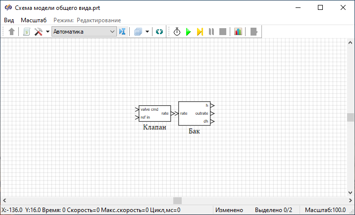
- Select from the drop-down menu the item General view model schematic
- Save the project, leaving the default name or specify the desired project name
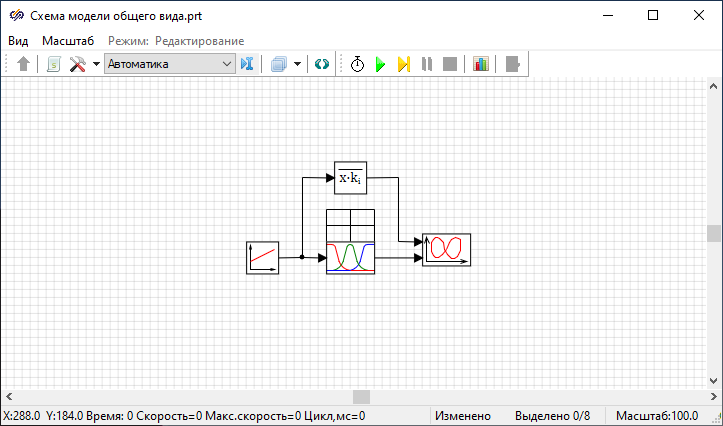
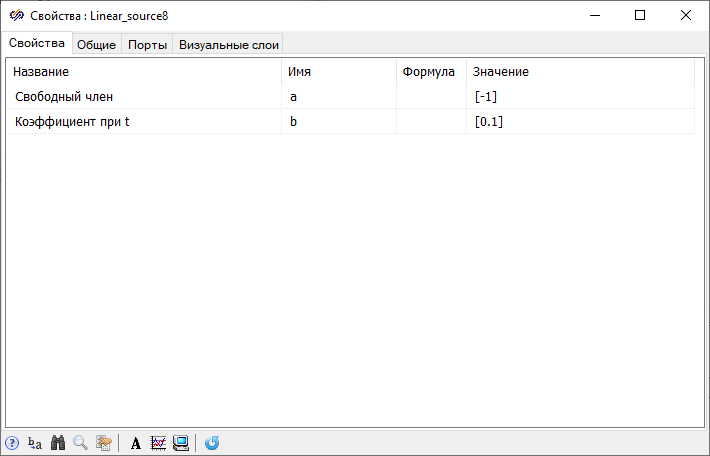
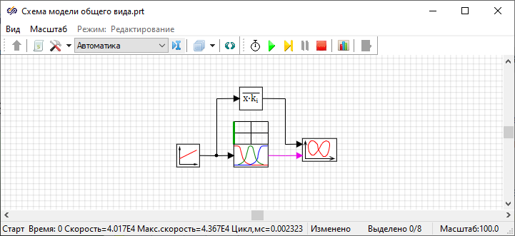
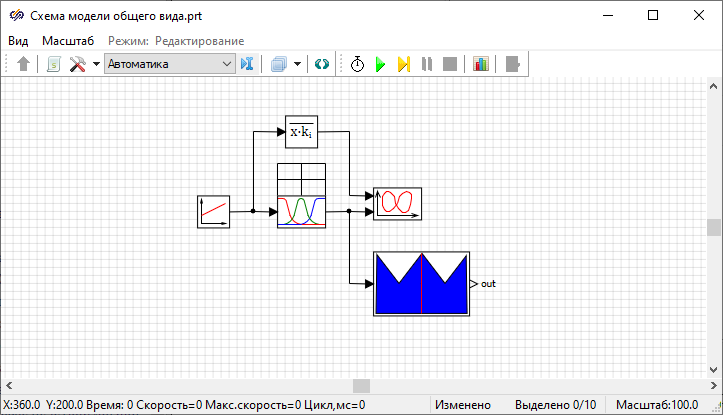
- 1 block Linear source from tab Sources – using this block, the values of the input variable x will be generated
- 1 block Vector replicator from tab Vector – using this block, the scalar signal will be converted into a vector of the required dimension
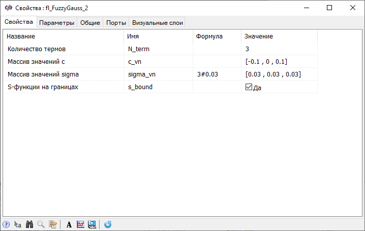
- 1 block Gaussian fuzzification from submenu Fuzzification of the tabFuzzy logic – using this block, the membership function values of the input variable x for each term will be calculated
- 1 block Phase portrait from tab Data output – using this block, a graphical display of the results of the work of Gaussian fuzzification will be performed
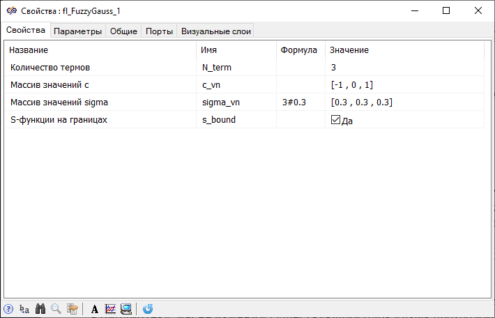
The property "S-function at the boundaries" is necessary to check the output of the input value outside the range, since the Gaussian function decreases outside the range, and therefore the value of the membership function decreases, which is not always permissible. For example, if the water temperature reaches 100°C, this should mean that the water is hot and it is necessary to open the cold water valve, but if the check for out of range is not carried out, then at this point the Gaussian function can have a value equal to 0, which will be interpreted as the water temperature is not hot, and subsequently can lead to incorrect results.
In order to draw three plots of membership functions on the same chart at once, to the inputs of the block Phase portrait three pairs of phase variables shall be transmitted, i.e. two vector values, of dimension "3”. To do this, it is necessary to convert the scalar input signal into a vector consisting of three identical elements equal to the input signal using a block Vector replicator. To do this, open the windowProperties of the block Vector replicator and in the "Formula" field, set the value of the "Multiplication coefficient" property to "3#1".
- "Maximum step" = "0.1"
- "End calculation time" = "20"
Starting the simulation and working with plots
After setting up the schematic, in order to plot the results of fuzzification, it is necessary to start the simulation process and wait for the end of the calculation.
- Open the window Plot properties of the block Phase portrait and set on tab Plots and axes names of plots in accordance with the specified terms: “low", "normal", "high" (Figure 5).
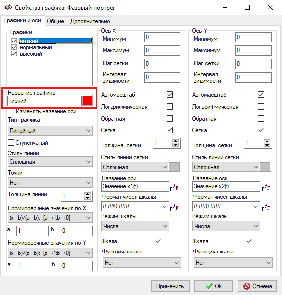
Figure 5. "Plot properties" window of the "Phase portrait" block with the property to be changed highlighted. - On tab General in the "Title" field, change the plot name to "Level"
Save changes and close the window by clicking the button Ok.
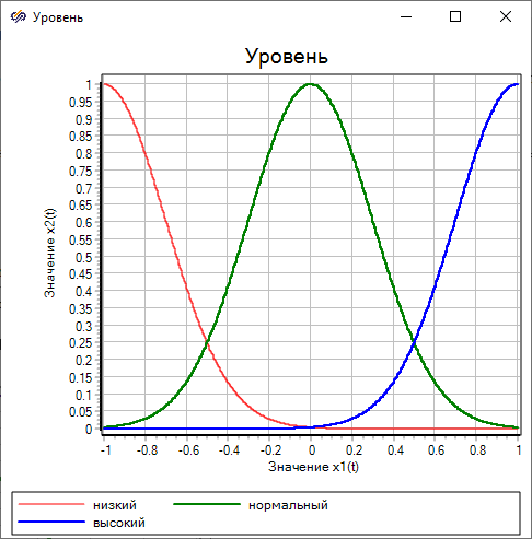
Plots of Gaussian membership functions are obtained, which show how a linear change in the input variable from -1 to 1 leads to a change in the values of three terms in the range from 0 to 1. At the beginning, when the input value is -1, the term "low" has a membership function equal to 1, the membership functions of the terms "normal" and "high" are zero. As the input value increases, the value of the membership function of the term "low" decreases, and the term "normal" begins to grow: the closer to 0, the closer the value of the function to 1. As the input value approaches 1, the membership function of the term "high" approaches 1, and the terms "low" and "normal" tend to 0. Thus, an increase in the input value from -1 to 1 is presented as a visual process of transition from "low", through "normal", to "high".
In addition to Gaussian fuzzification, it is possible to use blocks of triangular and trapezoidal fuzzification or, if the membership functions cannot be represented using these standard functions, it is possible to specify user-defined functions using a programming language. Example of implementing a two-sided Gaussian membership function using a block Programming language is given in Laboratory Work No.1 of the Moscow Polytechnic University "Study of the membership functions of fuzzy sets" in the section "Task 4. Plotting the two-sided Gaussian membership function. "
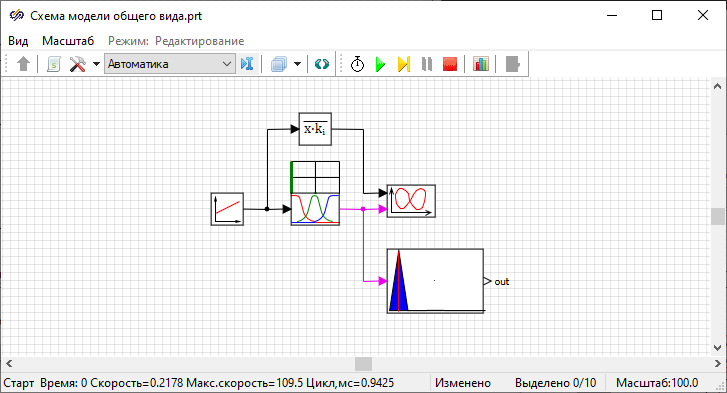
Study of the work of the "Gaussian fuzzification” animated block
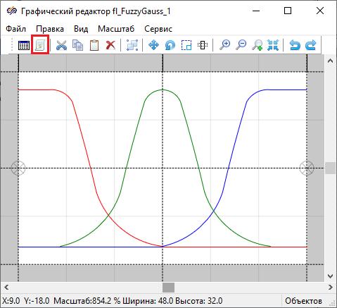
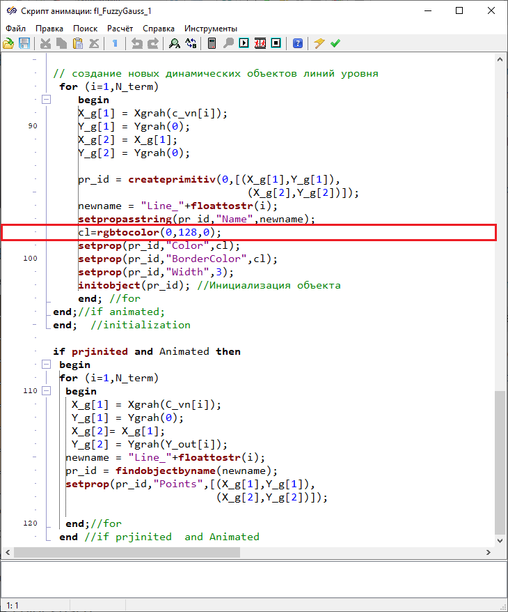
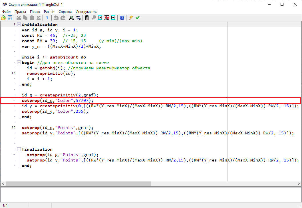
In the opened window Animation script the text of the script that changes the block image is included. For example, in the block animation script Gaussian fuzzificationcoordinates are calculated and new objects are set for display – grid lines of coordinate space, which are drawn above the block, as well as lines whose height varies depending on the values of the membership functions calculated during the simulation. By changing the animation script, you can change the display of existing image objects, for example, color or position, as well as add new objects.
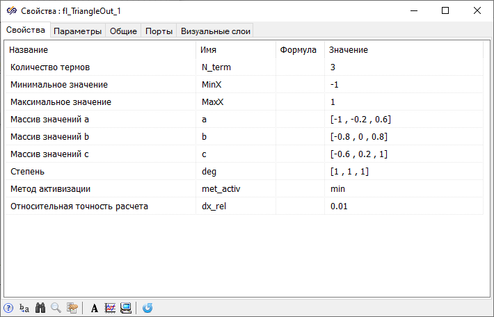
Addition to the model and study of the animated block "Triangular membership function block"
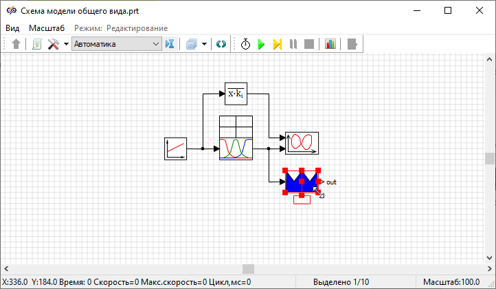
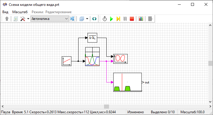
The model must be supplemented with a fuzzy inference system by adding a block that performs accumulation and defuzzification. To do this, add a block to the project window workspace. Triangular membership function block from submenu Fuzzy inferenceof the library Fuzzy logic and connect with a signal line according to figure (Figure 12).
Next, it is possible to track how the shapes and position of the line change either by setting a real-time synchronization or by performing a step-by-step simulation, as shown above.
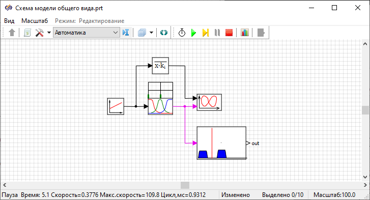
To view and edit the block animation script text Triangular membership function blockit is necessary to open the window Animation script in the same way previously described for the block Gaussian fuzzification.
In this task, the animation of blocks was considered using the example of library blocks Fuzzy logic. In addition to using standard blocks in SimInTech, it is possible to create your own blocks and it is also possible to make them animated. An example of creating a custom animation block and the procedure for adding it to a new library is described in SimInTech Laboratory work No.3 "Developing an animation block in SimInTech" (section "Developing a block library").
Familiarization with the work of animated blocks is completed. Further, using these blocks, a model of a leaky tank control system based on fuzzy logic will be developed.
Task 2. Development of a leaky tank control system based on fuzzy logic
In this task, a model of a leaky tank control system is considered, which should maintain the water level in the tank at a given level.
Leaky tank model description
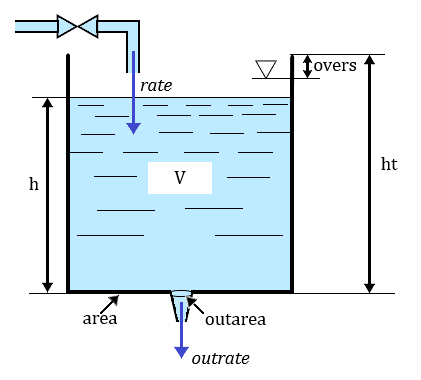
- "V" – tank volume, m3
- "ht" – tank height, m
- "area" – tank cross-section
- “outarea" – outlet hole area
- "overs" – position of the overflow sensor from the upper cut, m
- "h" – water level in the tank, m
- "rate" – flow rate entering the tank, m3/s
- "outrate" – outlet flow rate, m3/s
Leaky tank dynamics equations:
where g = 9.81 m/s2 is the acceleration of gravity.
Valve model description
- "0" – valve is closed – flow rate is zero
- "1" – the valve is opened – the flow rate is equal to the nominal one set as a constant
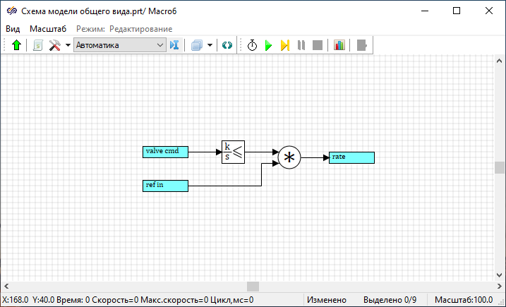
Output value – the flow rate of water entering the tank, "rate", is calculated as the product of the nominal flow rate and the valve position value.
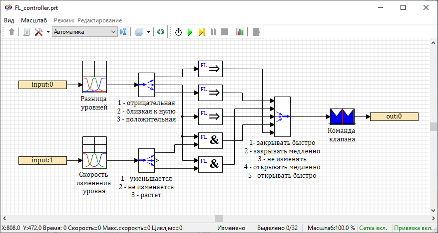
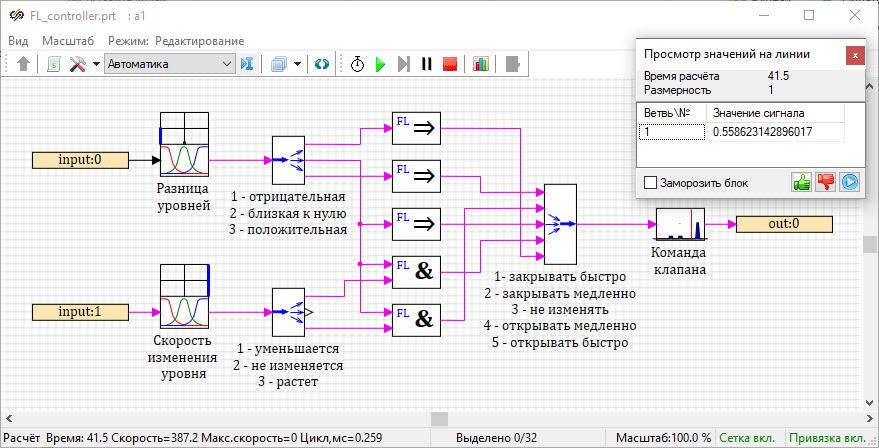
Fuzzy controller model description
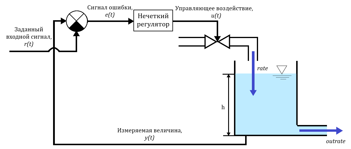
The controller is a fuzzy inference system that includes the following components: a fuzzifier, an inference engine, a defuzzifier.
- negative
- close to zero
- positive
Thus, if the difference between the current and target water level in the tank is negative, that is, the actual level is lower than the target, then it is necessary to increase the flow rate of water entering the tank; if the difference is positive, that is, the actual level exceeds the target, then it is necessary to limit the supply of water to the tank; if the difference is close to zero, that is, the actual level corresponds to the target or differs by a small amount, then it is not necessary to change the position of the valve, but if the water level changes with a certain speed, then to determine the opening/closing rate of the valve, it is necessary to take into account the second variable – "rate of level change".
- decreases
- does not change
- increases
So, if the level difference is close to zero and the rate of change of the level decreases, then it is necessary to slowly increase the flow of water entering the tank, and if the rate increases, then it is necessary to slowly reduce the flow of water entering the tank.
- close fast
- close slowly
- not to change
- open slowly
- open fast
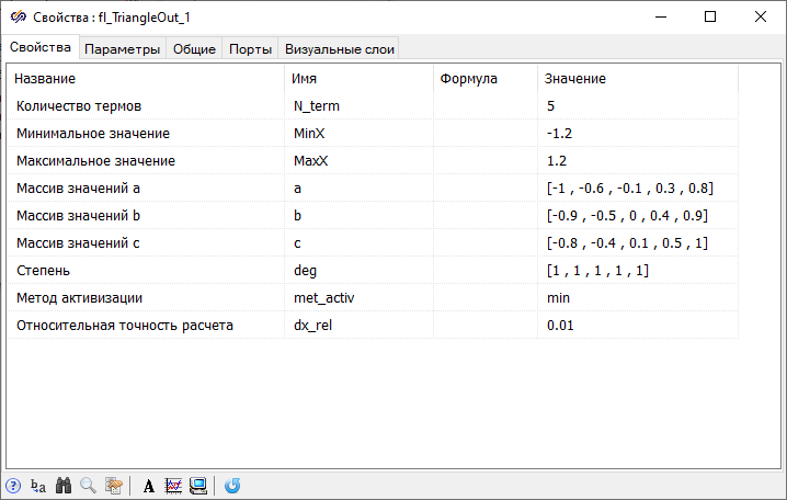
The membership functions that define fuzzy sets for input variables will be set as Gaussian membership functions, for the output variable – as triangular membership functions.
- IF "level difference" = "negative", THEN "valve control signal" = "open fast"
- IF "level difference" = "close to zero", THEN "valve control signal" = "do not change"
- IF "level difference" = "positive", THEN "valve control signal" = "close fast"
- IF "level difference" = "close to zero" AND "rate of level change" = "decreases", THEN "valve control signal" = "open slowly"
- IF "level difference" = "close to zero" AND "rate of level change" = "increases", THEN "valve control signal" = "close slowly"
Task accomplishment
- develop a model of a leaky tank
- develop a valve model
- develop a model of a fuzzy controller as the Mamdani fuzzy inference system
- simulate leaky tank control system
- draw the plots showing the dependence of water level in the tank over time and the dependence of outlet flow rate over time.
- compare the plots of the target and actual water level in the tank
Developing the model of a leaky tank
- In the main window of SimInTech, left-click the button File and select an item New project
- Select from the drop-down menu the item General view model schematic
- Save the project, leaving the default name or specify the desired project name
The development of models of a leaky tank, a valve and a fuzzy controller will be carried out in separate submodels for the convenience of organizing blocks according to models. After all models are developed, they will be combined into a general control system model.
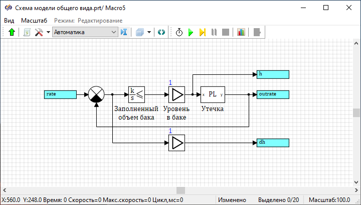
- 1 block Input port and 3 blocksOutput port from tabSubstructures – these blocks are designed to connect the external part of the diagram with the diagram inside the submodel
- 1 block Integrator with limitation and 1 block Programming language from tab Dynamic, 2 blocks Gain and 1 block Comparator from tab – these blocks simulate the operation of a leaky tank
initialization
    {Tank height}
    ht = 2;
    {Tank cross-section}
    area = 1;
    {Outlet pipe cross-section}
    outarea = 0.05;
    {position of the overflow sensor from the upper cut}
    overs = 0;
    {initial fluid level in the tank}
    inith = 0;
end; 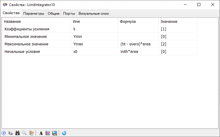
To set the formula for calculating the water level, open the window Properties of the blockGain labeled "Tank level" and set the "Gain factor" property to "1/area" in the "Formula" field.
{Calculation of tank leakage proportional to pressure}
input h;
g = 9.8;
outrate = sqrt(2*g*h)*outarea;
output outrate; 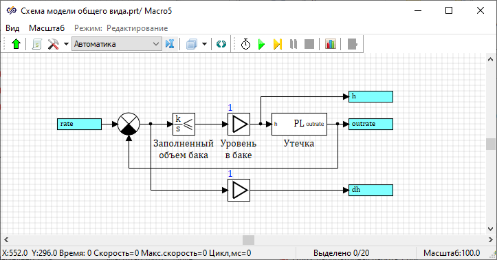
The creation of the tank model is completed, then you need to exit the submodel by double-clicking the left mouse button on the free space of the submodel workspace.
Developing the valve model
- 2 blocks Input port and 1 block Output port from tabSubstructures – these blocks are designed to connect the external part of the diagram with the diagram inside the submodel
- 1 block Integrator with limitation from tab Dynamic and 1 blockMultiplier from tab – these blocks simulate the operation of the valve
Developing the fuzzy controller model
- 2 blocks Input port and 1 block Output port from tabSubstructures – these blocks are designed to connect the external part of the diagram with the diagram inside the submodel
- 2 blocks Demultiplexer from tab Vector – this block allows you to divide the vector input signal into separate output signals
- 1 block Multiplexer from tab Vector – this block provides alternate transmission of several input signals to one output port
- 2 blocks Gaussian fuzzification from submenu Fuzzification of the tabFuzzy logic – these blocks are designed to fuzzification of the input signals, that is, to convert the crisp inputs of input values into fuzzy sets, determined using the values of the membership functions μA(error), μA(dh) corresponding to the given linguistic terms
- 3 blocks Implication, 2 blocks AND (conjunction) from submenuOperations of the tab Fuzzy logic – these blocks are designed to form an inference engine based on the rule base specified in the Fuzzy controller model description section
- 1 block Triangular membership function block from submenu Fuzzy inference of the tabFuzzy logic – this block is designed to defuzzify the output variable, that is, to convert a fuzzy set defined by the membership function μB(valve cmd) into a specific value of the output variable "valve cmd"
For blocks Demultiplexer it is necessary to set the value of the property "Array of input dimensions" to "[1, 1, 1]" and for the block Multiplexerto set the value of the property "Number of ports" to "5".
- IF "level difference" = "negative", THEN "valve control signal" = "open fast"
- IF "level difference" = "close to zero", THEN "valve control signal" = "do not change"
- IF "level difference" = "positive", THEN "valve control signal" = "close fast"
- IF "level difference" = "close to zero" AND "rate of level change" = "decreases", THEN "valve control signal" = "open slowly"
- IF "level difference" = "close to zero" AND "rate of level change" = "increases", THEN "valve control signal" = "close slowly"
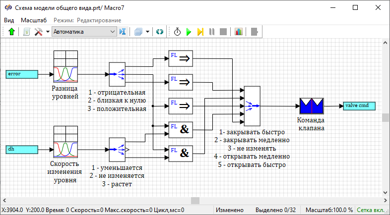
Labels for the blocks Demultiplexer and Multiplexer denote the correspondence between the numbers of output and input ports and linguistic terms. Thus, to the first output port of the upper block Demultiplexer corresponds the linguistic term "low", and to the first input port of the block Multiplexer corresponds the term "close fast".

After completing the configuration of the fuzzy controller model schematic, it is necessary to exit the submodel and resize the block labeled "Fuzzy controller" so that the port labels do not overlap each other.
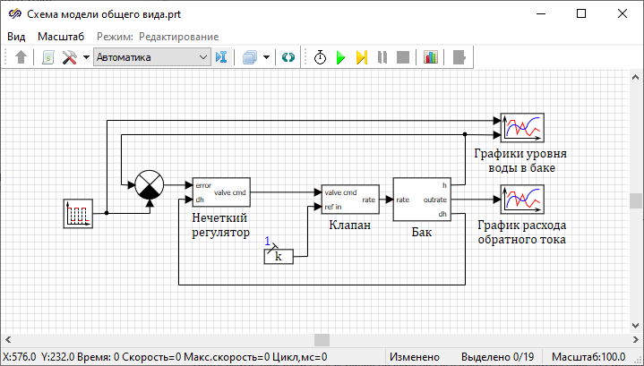
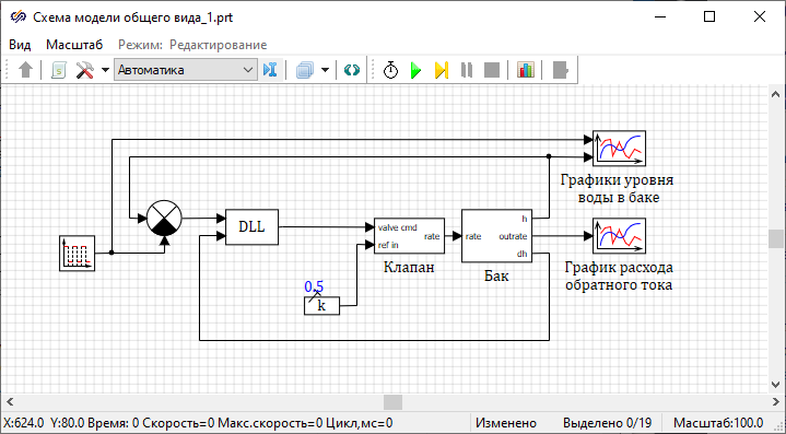
Merging the models into leaky tank control system based on fuzzy logic
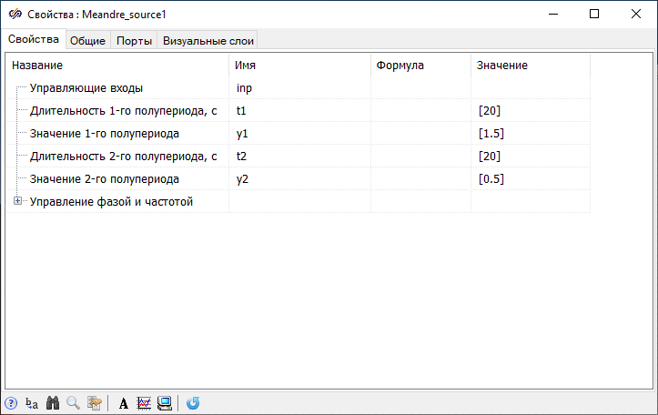
- 1 block Square wave from tab Sources – this block allows you to set the target water level with a certain frequency
- 1 block Constant from tab Sources – this block allows you to set the nominal flow rate of water entering the tank
- 1 block Comparator from tab – this block is designed to calculate the difference between the actual and target water level in the tank
- 2 blocks Scope from tab Data output – these blocks display the values of the simulation results in the form of plots
Since it is necessary to plot not only the actual water level, but also the target water level, and compare them, it is necessary that these plots be drawn in one window. This requires for one of the blocks Scope to set the value of the property "Number of input ports" to "2".
Next, you need to set the nominal flow rate of water entering the tank. To do this, open the window Properties of the block Constant and set the value of the "Value" property to "0.5".
Configuring simulation condition
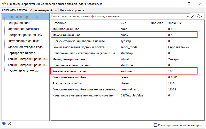
Close the window Project parameters, in this case the changes made are saved.
Starting the simulation and working with plots
After setting up the project for plotting, you need to start the simulation process and wait for the end of the calculation.
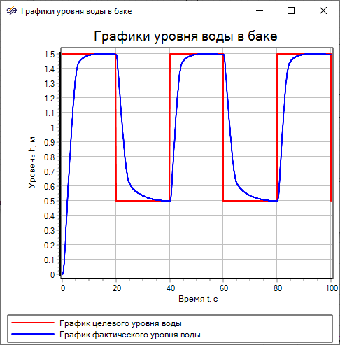
- Open the window Plot properties of the blockScope labeled "Plots of tank water level” and in the tab Plots and axes set the property values (Figure 35):
- in the "Plot name" field, set the name to the first plot "Plot of the target water level", name the second plot as "Plot of the current water level"
- in the "Y-axis" column, set the value of the "Axis name" property to "Level h, m"
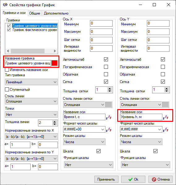
Figure 33. "Plot properties" window of the "Scope" block labeled "Tank water level plots" with the highlighted properties that need to be changed. - On tab General enter the plot name "Tank water level plots" in the "Title" field
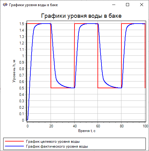
The plot of the target water level is pulses with a half-period of 20 seconds, the values of which will change from 1.5 m to 0.5 m and back. The plot of the current water level quite smoothly tends to the graph of the target level. As a result of the analysis of the obtained plots, it was proved that the model works correctly.
- Open the window Plot properties of the block Scope labeled "Plot of outlet flow rate” and set on the tab Plots and axesname of the Y-axis according to the figure (Figure 37).
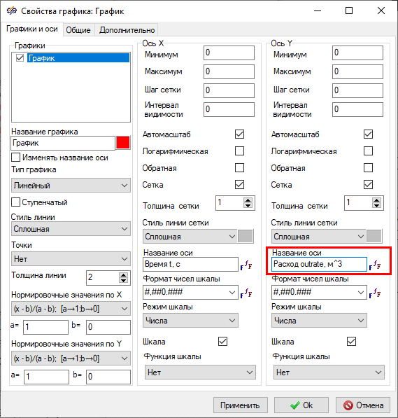
Figure 35. "Plot properties" window of the "Scope" block labeled "Plot of outlet flow rate" with the highlighted property that needs to be changed. - On tab General in the "Title" field, change the plot name` to "Plot of outlet flow rate" and disable the "Show legend" property (Figure 38).
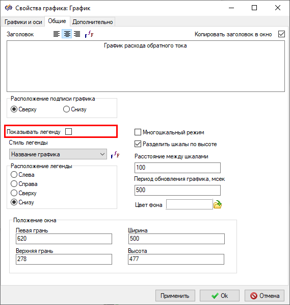
Figure 36. "Plot properties" window of the "Scope" block labeled "Plot of outlet flow rate", the tab "General" with the highlighted property that needs to be changed.
Save changes and close the window by clicking the button Ok.
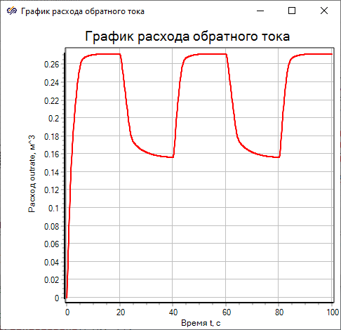
As a result of the analysis of the obtained plot, it was found that the plot fully corresponds to the expected results: the variable "outrate" at the time of 20 seconds is approximately equal to "0.271", which is consistent with the theoretical value calculated by the formula for the water level value at the same time equal to "1.5 m":
Task 3. Conversion of the control system of an leaky tank into a system with a fuzzy controller in the DLL form
SimInTech allows you to convert simulation diagrams of control algorithm models into dynamic-link libraries (DLL) using automatic generation of C code. The use of dynamic DLL libraries instead of the original schematics of control algorithm models allows you to significantly increase the simulation speed and check the performance of these algorithms as embedded control algorithms. This section is devoted to the conversion of the valve control algorithm – a fuzzy controller – into C program code and its compilation into DLL using a built-in template configured to create DLL libraries for Windows "MinGW".
- convert the fuzzy controller into a dynamic-link library view (DLL) using a code generator
- simulate the control system for the leaky tank with a converted fuzzy controller
- compare the results and speed of operation of the system model with the converted fuzzy controller and the original system model
Conversion of the fuzzy controller into a dynamic-link library (DLL) using a C code generator
Before converting the fuzzy controller into a dynamic-link library (DLL), it is necessary to save the model of the fuzzy controller to a separate file. To do this, double-click with the left mouse button on the block Submodel labeled "Fuzzy controller” to enter the submodel, then in the main window of SimInTech you need to select the item File subitemSave page as. Save the fuzzy controller model to a new project file named "FL_controller.prt".
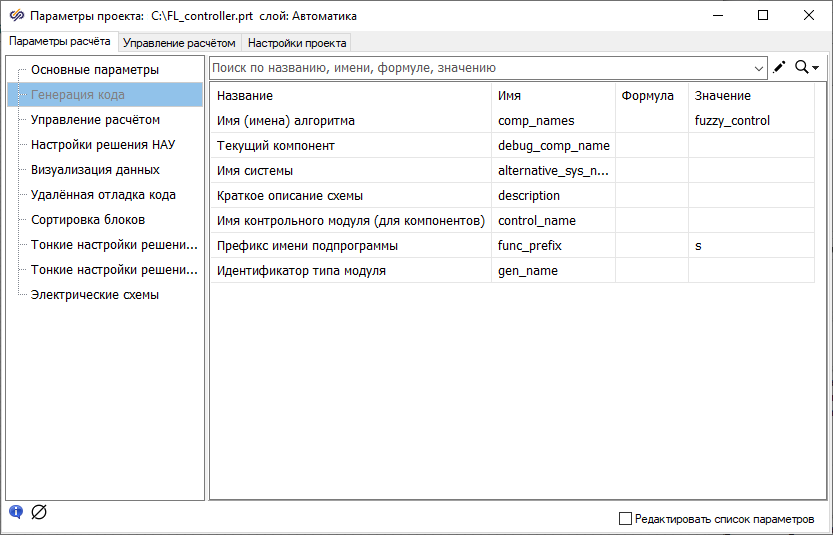
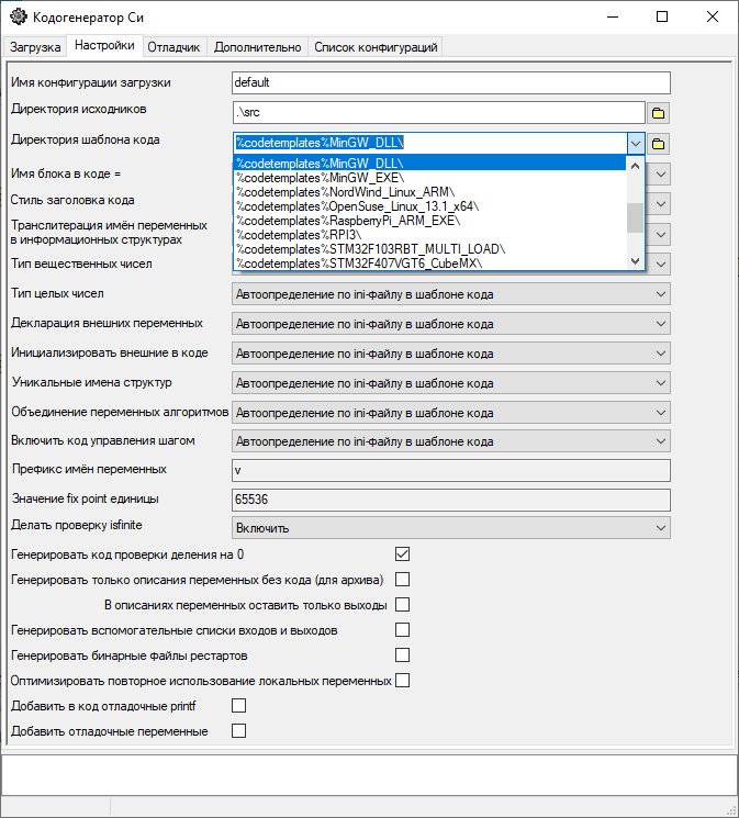
In particular, for example, to obtain code that performs calculations with a fixed point, it is necessary in the tab Settings in the "Code template directory" line, select the line in the drop-down menu: "%codetemplates%FixPoint_16_16_MinGW_DLL\".
- <algorithm name>.h
- <algorithm name>.inc
- <algorithm name>.log
- <algorithm name>_init.inc
- <algorithm name>_state.inc
- <algorithm name>.dll
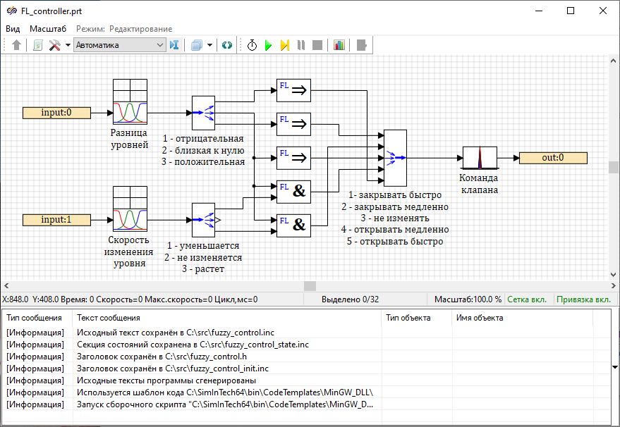
Figure 42. Project workspace with code generator messages for the diagram.
Study the operation of the control system of the leaky tank with the fuzzy controller in the DLL form
To study the operation of the control system of the leaky tank with the fuzzy controller in the DLL form, it is necessary to save a copy of the project with the original model of the system "General view model schematic.prt" using the name "General view model schematic_1.prt". Open the project "General view model schematic_1.prt".
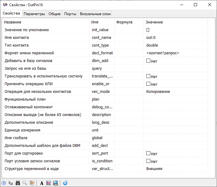
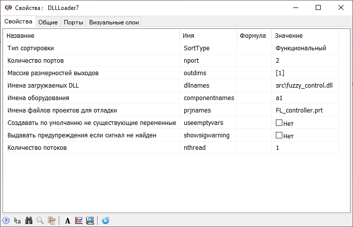
- "Number of ports" – using this property, the number of input ports of the block is set in accordance with the number of input contacts in the simulation diagram of the fuzzy controller "FL_controller.prt"
- "Array of output dimensions" – with the help of this property, the dimensions of the output ports are set in the form of an array, and the dimension of the array corresponds to the number of output contacts in the simulation diagram of a fuzzy controller. After closing the window and saving the properties to the block DLL two input ports and one output port will appear
- "Names of loaded DLLs" – this property sets the path to the file generated in the previous step with the ".dll" extension
- "Project file names for debugging" – this property specifies the name of the project file with the fuzzy controller simulation diagram corresponding to the loaded DLL that can be used to debug the schematic. To monitor the process of simulating the fuzzy controller, it is necessary to set real-time synchronization. To proceed this, open the window Project parameters and in the tab Simulation control activate the parameterReal-time synchronization, and after starting the simulation, double-click with the left mouse button the blockDLL, then the project specified in the value of this property will open
- "Sorting type" – using this property, a checkbox is set that defines the simulation order in the main diagram
- "Equipment names" – with the help of this property, the names of equipment (components) are set, which are substituted into the input/output contacts of the DLL schematic
- "Create non-existing variables by default" – when this property is activated, variables will be created in the database that do not exist for the calculated equipment (components)
- “Issue warnings if the signal is not found" – when this property is activated, warnings will be issued if the signal is not found
- "Number of threads" – this property sets the number of threads in which simulations will be made for this DLL


Conclusion
In the course of this laboratory work, a model was developed for studying the operation of animated blocks on the example of the blocks of the library Fuzzy logic. A model of the control system for the leaky tank with the controller based on the Mamdani type fuzzy inference system the was also developed. The plot of the dependence of the water level in the tank on time and the outlet flow rate on time were drawn, and the plots of the target and current water level in the tank were compared. As a result of mathematical modeling, the correctness of the operation of the control system model of the leaky tank based on fuzzy logic was tested.
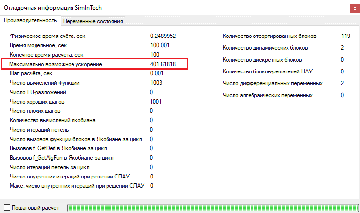
To get acquainted with the methods of C-code generator operation, the conversion of the fuzzy controller into the dynamic-link library (DLL) was carried out. The test simulation showed that the fuzzy controller in the form of a dynamic DLL generated in C language works similarly to the fuzzy controller in the submodel. Comparison of operating speedups showed that a system with a controller in the DLL form works several times faster than a similar system with a controller in the form of a schematic in a submodel.