Timeline
 |
 |
| Vectorized | |
in the palette |
on the schematic |
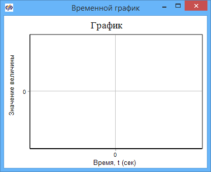
The block implements the display of current simulation results in the form of time dependencies for one or for several variables simultaneously. It can be used both for local simulation and remote debugging to display the values of signals calculated on the target system. In the Schematic window the block image is similar to the image of any typical block - a rectangle with a characteristic icon. If you click 2 times with the left mouse button on the block image in the schematic window, the so-called graphic window opens (it is also opened when initially placing the block on the schematic):
Inputs
- inport_n - input port. The number of input ports and, therefore, the values displayed on the plot are set in the block properties.
Outputs
None
Properties
- The Number of input ports is the number of block ports, the default is 1; in other words, the number of signals (scalars or vectors) displayed in the graphic window.
Parameters
- The Total input vector is a one-dimensional array that shows the current signal values on all input ports.
Additional settings
When you right-click on the graphic window, a drop-down menu will appear with the Properties menu item, as well as with the following options:
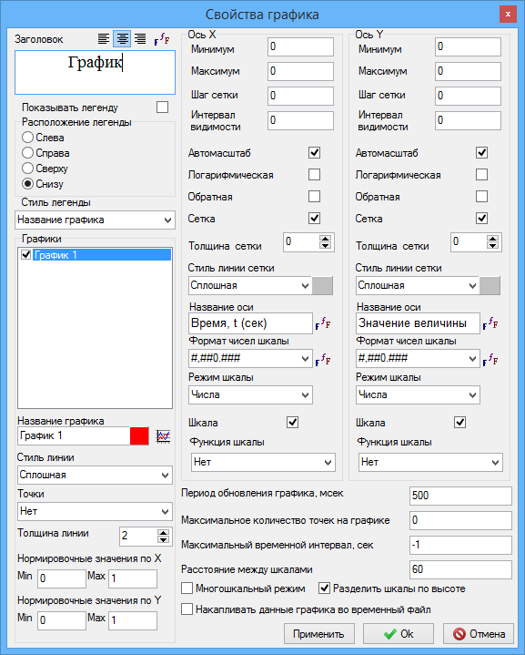
It is better to study all the features of this window yourself. The most frequently used settings are: - Plot background - select the fill color of the plot background (white by default);
- Underlay – select a bitmap image as the background of the graph; the image will be scaled to the size of the graph;
- Window dimensions - setting the exact width and height of the graphic window in pixels;
- Copy to clipboard - copy the image of the graphic window to the clipboard for pasting into other programs (Paint, Word, Photoshop, AutoCAD...);
- Export to file - save the image in one of the common graphic formats;
- Print - print the graph;
- Table - change the method of displaying the time dependence to a tabular one (reverse switching is similar);
- Save to a text file - save the function of time to a folder file in a tabular form;
- Export to Excel – export the function of time in tabular form to MS Excel;
- Cursor - an additional opportunity for an accurate study of the displayed function of time;
- On top of all windows - if enabled, the plot is displayed on top of all other windows;
- Subsample points - if enabled (by default yes), the displayed data is subsampled according to the following algorithm: if 3 consecutive calculation points lie on the same line (with a given accuracy), then the midpoint is not displayed on the plot, since the segment drawn through the 1st and 3rd points also contains the 2nd point. If it is necessary to have information about all calculation data displayed on the chart, you should uncheck (turn off) this option;
- Delete invisible points - if enabled (by default yes), then those calculated data (plot points) that have undergone subsampling will be deleted from RAM and from the plot. This procedure avoids excessively large data sets accumulated in computer memory when simulating long transients.
- Plot name is the name of the plot in the legend;
- Line style is a style of the line that displays the selected function of time;
- Line thickness is a thickness in pixels of the line of the selected plot;
- Title - the name of the plot (at the top), you can set the font parameters;
- Axis name - a text line displayed near the axis with the name of this axis;
- Autoscale is the ability to autoscale (or not) a plot. By default, autoscaling is enabled;
- Plot update time - If you are researching long processes, it is helpful to increase the update period. If the processes under study are short, it is better to reduce this parameter.
- Multi-scale mode - the ability to display different scales to display different values.
A video tutorial on capabilities of configuring plots is available xref href="https://www.youtube.com/watch?v=uqvJA7lTtJk" format= "html" scope= "external">at link/xref.