Mikhailov Locus


`in the palette`	`on the schematic`

The block forms the Mikhailov locus for the closed dynamic control system that is in the project. When installing the block on the schematic, a graph window is created, in which the locus will be displayed.

The work of the block is based on the criterion formulated in 1938 by the Soviet scientist Mikhailov A.V., which makes it possible to judge the stability of systems based on the consideration of a curve called the Mikhailov curve.

The polynomial of the left part of the differential equation of the closed system, or the denominator of the transfer function of the closed system is the initial characteristic polynomial of the closed system:

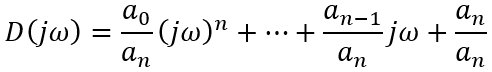
If we substitute a purely imaginary value of s = jω in this polynomial, we get a complex polynomial called the Mikhailov polynomial:

When the frequency ω changes, the vector D(jω), changing in magnitude and direction, will describe with its end in the complex plane a curve called the Mikhailov curve (locus).

Mikhailov's stability criterion can be formulated as follows. In order for the automatic control system to be stable, it is necessary and sufficient that the Mikhailov curve (locus), when changing the frequency from 0 to +∞, starting at ω = 0 on the real positive semi-axis, bypasses only counterclockwise successively n quadrants of the coordinate plane, where n is the order of the characteristic equation.

The Mikhailov curve for stable systems always has a smooth spiral shape, and its end goes to infinity in the quadrant of the coordinate plane, the number of which is equal to the order of the characteristic equation (polynomial degree).

A sign of the instability of the system is a violation of the number and sequence of the Mikhailov curve quadrants of the coordinate plane, as a result of which the angle of rotation of the vector D(jω) is less than n∙(π/2).

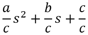
Прим.: When forming the Mikhailov locus, the values of the function are reduced to a certain range or scale, that is, the function graph is normalized. Normalization of the function graph is achieved by bringing the values to a certain range by dividing all the coefficients of the polynomial by its last free coefficient. Thus, the plotting is carried out according to the following function:

If the transfer function has the form: as² + bs + c, the graph of the function will be normalized by the coefficient c:

Ports

The block has no input and output ports. There is analyzed the closed dynamic control system that is being designed.

Properties

Title	Parameter	Description	By default	Data type
Starting circular frequency, 1/sec	wstart	Indicates the beginning of the range of circular frequencies in which the Mikhailov polynomial will be calculated	0.5	Real
End circular frequency, 1/sec	Wend	Indicates the end of the circular frequency range in which the Mikhailov polynomial will be calculated	20	Real
Number of output points	ptcount	Number of values of circular frequencies within the range for which the Mikhailov polynomial will be calculated (number of plot points)	500	Integer
Relative increment for Jackobian	dJotn	The value used for carrying out linearization of nonlinear objects	0.001	Real
Absolute increment for Jackobian	dJabs	The value used for carrying out linearization of nonlinear objects	1E-6	Real
Characteristics calculation mode	ffdcalcmode	It allows us to determine a moment of calculation: during schematic initialization, when the final calculation time is reached or with a preset step (i.e. "At the beginning of calculation", "At the end of calculation", "With a preset step")	At the beginning of calculation	Enumeration
Characteristics calculation step, sec	ffdtimestep	The value of the time step with which the characteristics are recalculated. The property is used if the "With a preset step" mode is selected	0	Real

Прим.: property window is opened via context menu of the block

Parameters

Title	Parameter	Description	Data type
X values	X	Array of real parts of the Mikhailov polynomial at each output point	Array
Y values	Y	Array of real parts of the Mikhailov polynomial at each output point	Array

Examples

Examples of block application: