Plotting of the transfer functions
 |
 |
| Vectorized | |
in the palette |
on the schematic |

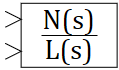
where N(s) and L(s) are characteristic polynomials of the system, as well as in the form of matrices of equations of state of a linear continuous system of the following form:
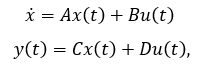
where  is the time derivative of the vector x(t);
x(t) is a state vector of dimension (n×1), the components of which are state variables of the n-th order system;
A is a matrix of system coefficients, dimension (n×n);
B – input matrix, dimension (n×r);
u(t) is an input vector of dimension (r×1), the components of which are the input variables of the system (r);
y(t) is the output vector of dimension (p×1), the components of which are the output variables of the system (p);
C – output matrix, dimension (p×n);
D is a detour matrix with dimension (n×r), which determines the direct dependence of the output on the input.
Both the coefficients of the transfer function and the set of matrices of the state equations system are individually equivalent full-fledged representations of the mathematical description of a dynamic object.
The output calculated values are displayed in the form of a table that opens when you double-click the left mouse button on the block image.
Input Ports
| Parameter | Description | Communication line type |
|---|---|---|
| in | Port for connection of the output signal of the object under study | Mathematical |
| out | Port for connection of the input signal of the object under study | Mathematical |
Output Ports
The block has no output ports
Properties
| Title | Parameter | Description | By default | Data type |
|---|---|---|---|---|
| Relative increment for Jackobian | dJotn | The value used for carrying out linearization of nonlinear objects | 0.001 | Real |
| Absolute increment for Jackobian | dJabs | The value used for carrying out linearization of nonlinear objects | 1E-6 | Real |
| Characteristics calculation mode | ffdcalcmode | It allows us to determine a moment of calculation: during schematic initialization, when the final calculation time is reached or with a preset step (i.e. "At the beginning of calculation", "At the end of calculation", "With a preset step") | With a preset step | Enumeration |
| Characteristics calculation step, sec | ffdtimestep | The value of the time step with which the characteristics are recalculated. The property is used if the "With a preset step" mode is selected | 0 | Real |
| Reduce degree of the numerator and the denominator polynomials | ReduceDeg | Checkbox to activate degree reducing of the numerator and the denominator polynomials | Yes | Binary |
| Absolute comparison accuracy of the roots of the numerator and the denominator when reducing degrees of polynomials | ReduceTol | Absolute allowable error in comparison of the roots of the numerator and the denominator when reducing degrees of polynomials. This option is available in the property "Reduce degree of the numerator and the denominator polynomials" | 1E-5 | Real |
Parameters
| Title | Parameter | Description | Data type |
|---|---|---|---|
| Numerator W(s) | Ns | Array of coefficients bi of the numerator polynomial of the form N(s)=b0sm+b1sm-1+...+bm starting from bm | Matrix |
| Denominator W(s) | Ls | Array of coefficients ai of the denominator polynomial of the form L(s)=a0sn+a1sn-1+...+an starting from an | Matrix |
| Zeros (roots of equation N(s) = 0) | Zeros | Array of zeros of the transfer function (the roots of the characteristic polynomial in the numerator of the transfer function) | Complex matrix |
| Poles (roots of equation L(s) = 0) | Poluses | Array of transfer function poles (characteristic polynomial roots in the transfer function denominator) | Complex matrix |
| Matrix A (eigenmatrix) | A | Value of the eigenmatrix of the state equations system | Matrix |
| Matrix B (input matrix) | B | Value of the matrix of inputs of the state equations system | Matrix |
| Matrix C (output matrix) | C | Value of the matrix of outputs of the state equations system | Matrix |
| Matrix D (detour matrix) | D | Value of the detour matrix of the state equations system | Matrix |
Examples
Examples of block application: