Optimizer

		`\| Vectorized \|`
`in the palette`	`on the schematic`	`\| Vectorized \|`

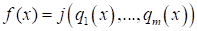
The optimizer block is intended for picking up such optimization parameters, that would satisfy the required values of optimization criteria

Thus, optimization task might be formulated as finding of the optimization parameters vector at which quality criteria meets their limits.

The optimization problem is difficult to formalize, therefore, in order to obtain any effective results, a set of optimization criteria and parameters having different physical nature and ranges of change must be scaled and converted to normalized values.

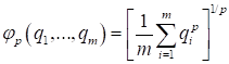
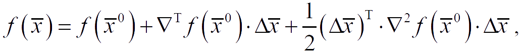
In the presence of a set of criteria, to formalize the conditions of the optimization problem, they usually go from several partial criteria q₁, …, q_m to one general criterion, which is formed as a function of partial criteria. This procedure is called criteria folding. The result is a general criterion (goal function):

as a function of the optimized parameters. The solution of the multi-criteria optimization problem is reduced to minimizing this criterion. One of the most commonly used methods of folding of partial criteria is the average power criterion of optimality. This is what is used to fold the optimization criteria in SimInTech:

For p = 2, the criterion is quadratic:
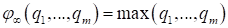
When p tends to infinity, the general criterion is reduced to the largest of the standardized partial criteria (minimax criterion):
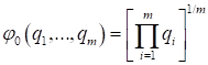
With p = 0, logarithmizing the expression of the general criterion and moving to the limit on p, which tends to zero, after applying the L'Hopital's rule, the average geometric (multiplicative) optimality criterion will be obtained:

Having obtained a generalized criterion, you can begin to solve the optimization problem.

Optimization algorithms

SimInTech implements 5 optimization algorithms most suitable for software implementation, in which the decision to move to a new search point is made on the basis of comparing the values of the criterion at two points.

Algorithm Search-2

An algorithm for dividing the step in half with one optimized parameter (n = 1) and an algorithm for transforming the direction matrix at n > 1 are implemented.

Next, we consider the multivariable search algorithm.

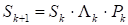
The search directions at the k-th stage are set by the matrix S_k. At the next stage, a series of descents is made in the directions of vectors s₁, …, s_n, which are columns of the matrix S_k. The displacement vectors on each of the descents are respectively g₁s₁, …, g_ns_n. After the descents are made, the matrix of directions is transformed according to the formula:

where Λ_k is a diagonal matrix whose elements are equal to λ_k = γ_i if γ_i ≠ 0, and λ_k = 0.5 if γ_i = 0; P_k is an orthogonal matrix.

Multiplication by an orthogonal matrix is necessary to change the set of search directions. If at all stages P_k = i, then the search directions do not change from stage to stage and the algorithm is a coordinate descent algorithm. Obviously, the choice of P_k matrices significantly affects the search efficiency.

Several different ways of selecting orthogonal matrices P_k have been tested, including random selection. The best was the way in which all matrices P_k are equal to each other and are defined in the form:

Steps of the algorithm in the multivariable case:

The initial matrix of directions is given by the diagonal one with elements on the main diagonal equal to the initial increments in terms of parameters.
Running cycle for i = 1, …, n:
1. A trial step is performed in the direction of s_i: y = x + s_i.
  If this step is successful (f(y) < f(x) ), proceed to point c.
2. Then a trial step in the opposite direction is performed: y = x − s_i.
  If both trial steps were unsuccessful, λ = 0.5 is taken and the transition to point d is performed.
3. Descent is performed in the selected direction, as a result, a new search point x = x + γs_i will be obtained, λ = |γ| is taken.
4. Accept s_i = λs_i. Go to the next cycle counter value or exit the cycle (if i = n).
Multiplication of the matrix of directions S by the orthogonal matrix P given by the expression.
When the search end condition is met, the algorithm closes, otherwise - the transition to item 2 with the new values of the vector x and the matrix S.

The search is terminated if one of the following conditions is met:

the goal function has reached the minimum (all requirements are met);
the specified number of calculations of the goal function is exceeded;
increments for each of the parameters are less than the set value;
forced stop.

Algorithm Search-4

The quadratic interpolation algorithm is implemented with one optimized parameter (n = 1) and the algorithm of rotation and stress-strain transformations (n > 1).

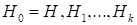
Algorithm at n > 1. The algorithm is based on performing stress-strain transformations and rotation transformations for such a transformation of the coordinate system, in which the matrix of the second derivatives (Hessian matrix) approaches the unit one, and the search directions become conjugate. This algorithm uses quadratic interpolation.

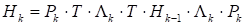
Let H be a symmetric positively definite matrix. A sequence of matrices is formed:

each of which is obtained from the previous one by performing the following transformation:

where Λ_k is a diagonal matrix with elements λ_i = h_ii−1/2 (h_ii are diagonal elements H_k_-1); P_k is an orthogonal matrix.

After pre-multiplying and post-multiplying the matrix H_k−1 by Λ_k, a matrix with unit diagonal elements is obtained. With a suitable choice of orthogonal matrices P_k, the matrix H_k will tend to be the identity matrix. On this, in particular, the method of rotations for calculating the eigenvalues of symmetric matrices is based.

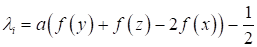
In the problem of finding the minimum of the function of several variables at the k-th stage of the search, the function is alternately minimized in the directions of vectors s₁,…, s_n, which are columns of the matrix S_k. To find the minimum point in the direction s_i, quadratic interpolation is used over three equidistant points z = x − as_i, x , y = x + as_i.

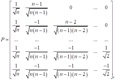
Simultaneously for each direction is calculated

After a series of descents, the matrix S is transformed according to the formula:

where Λk is a diagonal matrix, the elements of which are determined by the expression; P_k is some orthogonal matrix.

For a quadratic goal function, the matrix S_kT H S_k, where H is the Hesse matrix, coincides with the matrix H_k. Thus, with proper selection of matrices P_k for the quadratic function S_kT H S_k → i and the search directions approach the conjugates. In the algorithm under consideration, the matrices P_k are equal at all stages and are determined by the formula.

The steps of the Search-4 algorithm are similar to the steps of the Search-2 algorithm discussed above.

Simplex Algorithm

The "flexible polyhedron" method of Nelder and Mead is used.

In the Nelder-Mead method, the function of n independent variables is minimized using n+1 vertices of the flexible polyhedron. Each vertex can be identified by a vector x. The vertex (point) at which the value of f(x) is maximum is projected through the center of gravity (centroid) of the remaining vertices. The improved (smaller) values of the goal function are successively replaced by a point with a maximum value of f(x) for more “good” points until a minimum of f(x) is found.

The essence of the algorithm is summarized below.

Let x_i(k) = [x_i1(k), …, x_ij(k), …, _{x in}(k)]T, i = 1, …, n+1, be the i-th vertex (point) at the k-th stage of the search, k = 0, 1, …, and let the value of the goal function in x_i(k) be equal to f(x_i(k)). Polyhedron vectors that give maximum and minimum values are also noted.

Let f(x_h(k)) = max{f(x₁(k)), …, f(x_n+1(k))},

where x_h(k) = x_i(k) , and

f(x_l(k)) = min{f(x₁(k)), …, f(x_n+1(k)),

where x_l(k) = x_i(k).

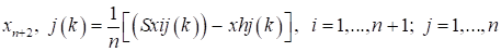
Since the polyhedron in E_n consists of (n+1) vertices x₁, …, x_n₊₁, let x_n₊₂ be the center of gravity of all vertices except x_h.

Then the coordinates of this center are determined by the formula:

where index j denotes the coordinate direction.

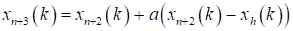
The initial simplex is usually (but not always) selected in the form of a regular simplex, and the origin of the coordinates can be placed in the center of gravity. The procedure for finding a vertex in E_n, in which the f(x) has the best value, consists of the following operations:

Reflection - designing x_h(k) through the center of gravity according to the expression:

where a is the reflection coefficient; x_n+2(k) is the center of gravity calculated by the formula; x_h(k) is the vertex in which the function f(x) takes the largest of n+1 of its values at the k-th stage.
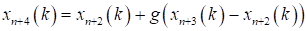
Strain. This operation is as follows: if f(x_n+3(k)) <= f(x_l(k)), then the vector (x_n+3(k) − x_n+2(k)) is strained according to the relation:

where g >1 is the strain coefficient.

If f(x_n+4(k)) < f(x_l(k)) , then x_h(k) is replaced by x_n+4(k) and the procedure continues again staring from the operation 1 at k = k+1. Otherwise, x_h(k) is replaced by x_n₊₃(k) and the transition to operation 1 is also carried out at k = k+1.
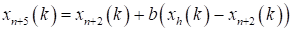
Stress. If f(x_n+3(k)) > f(x_i(k)) for all i < > h, then the vector (x_h(k) − x_n₊₂(k)) is stressed according to the formula:
where 0 < b <1 is the stress coefficient.
Then x_h(k) is replaced with x_n+5(k) and we return to the operation 1 to continue the search at (k+1) step.
Reduction. If f(x_n+5(k)) > f(x_h(k)), all vectors (x_i(k) − x_l(k)), i = 1, …, n +1, are reduced by 2 times starting from x_l(k) according to the formula:
Then goes on returning to the operation 1 to continue the search in (k + 1) step.

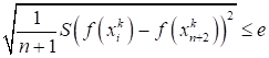
The criterion for the end of the search is to check the following condition:

where e is an arbitrary small number, and f(x_n+2(k)) is the value of the goal function in the center of gravity x_n₊₂(k).

The optimization process is influenced by the coefficients of a reflection a, a strain g and a stress b:

The reflection coefficient a is used to design the vertex with the highest value f(x) through the center of gravity of the flexible polyhedron.
The coefficient g is introduced to strain the search vector if the reflection gives a vertex with a value f(x) less than the smallest value f(x) obtained before the reflection.
The stress coefficient b is used to reduce the search vector if the reflection operation did not result in a vertex with a value f(x) less than the second largest (after the largest) value f(x) obtained before reflection.

Thus, by means of strain or stress operations, the dimensions and shape of the flexible polyhedron are scaled so that they satisfy the topology of the problem being solved.

After the flexible polyhedron is suitably scaled, its dimensions must be kept constant until changes in the topology of the problem require the use of a polyhedron of a different shape. The analysis conducted by Nelder and Mead showed that the compromise value is a = 1. They also recommend values of b = 0.5, g = 2. More recent studies have shown that ranges of 0.4 ≤ b ≤ 0.6, 2.8 ≤g ≤ 3.0 are recommended, with 0 < b < 0.4 likely to result in a premature end to the process due to polyhedron flattening, and b›0.6 may require more steps to reach a final solution.

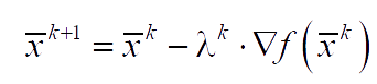
Algorithm for the fastest descent

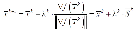
The gradient of the function at any point shows the direction of the greatest local increase f(x̅). Therefore, when searching for the minimum of f(x̅), one should move in the direction opposite to the direction of the gradient ∇f(x̅) at a given point, i.e., in the direction of the fastest descent. The iterative formula of the process of the fastest descent is as follows:

Obviously, depending on the choice of the parameter λ, the descent trajectories will differ significantly. When λ is large, the descent trajectory will be an oscillatory process, and when λ is too large, the process may diverge. When selecting small λ, the descent trajectory will be smooth, but the process will converge very slowly. Typically, λ is selected from the condition:

solving a single-variable minimization problem using some method. In this case, the algorithm is the fastest descent algorithm. If λ is determined by single-variable minimization, then the gradient at the point of the next approximation will be orthogonal to the direction of the previous descent ∇f(x̅)⟂S̅^k.

Conjugate gradient method

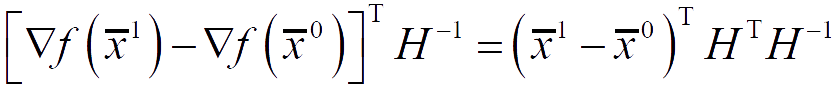
The fastest descent algorithm uses only the current information about the function f(x̅^k) and the gradient ∇f(x̅^k) at each search step. The algorithms of conjugate gradients use information about the search at the previous stages of descent.

The search direction S̅k at the current step k is constructed as a linear combination of the fastest descent −∇f(x̅^k) at the current step and the descent directions S̅⁰, S̅¹, …, S̅^k−1 at previous steps. The weights in the linear combination are selected in such a way as to make these directions conjugate. In this case, the quadratic function will be minimized in n steps of the algorithm.

When selecting weights, only the current gradient and the gradient at the previous point are used.

At the starting point x̅⁰, the descent direction is S̅⁰ = −∇f(x̅⁰) :

where λ⁰ is selected from the considerations of the minimum of the goal in this direction:

New search direction:

where ω₁ is selected so as to make the directions S̅¹ and S̅⁰ conjugate with respect to the matrix H:

For a quadratic function, the following relations are valid:

where Δx̅ = x̅ − x̅⁰,

If we take x̅= x̅¹, then x̅¹ − x̅⁰ = λ⁰S̅⁰ and

Using the expression above, it is possible to exclude (S̅⁰)^T from the equation. For the quadratic function H = H^T, therefore, after transposing the expression and post-multiplying by H⁻¹, the following expression is obtained:

and then

Consequently, for the conjugation of S̅⁰ and S̅¹we have:

Due to the conjugacy properties described earlier, all cross terms disappear. Taking into consideration that S̅⁰ = −∇f(x̅⁰) and therefore,

the following ratio is obtained for ω₁:

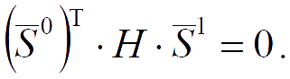
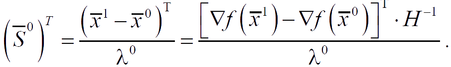
The search direction S̅² is constructed as a linear combination of the vectors −∇f(x̅²), S̅⁰, S̅¹, such that it is conjugate to S̅¹.

If we extend the calculations made to S̅², S̅³, …, omitting their content and taking into account that (S̅^k)^T∇f(x̅^k+1) = 0. That leads to ∇^Tf(x̅^k)∇f(x̅^k+1) = 0, we can obtain the general expression for ω_k:

All the weight coefficients preceding ω_k, which is especially interesting, turn out to be zero.

The algorithm is fully described by the following sequence of actions:

At the initial approximation point x̅⁰ S̅⁰ = ∇f(x̅⁰) is calculated.
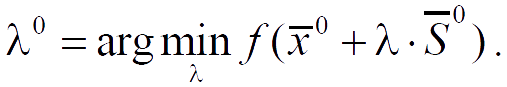
At the k-th step, using a single-variable search in the directionS̅^k, the minimum of the function is determined, that is, the problem is solved:
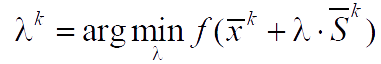
and there is another approximation x̅^k+1 = x̅^k + λ^k · S̅^k.
f(x̅^k+1) и ∇f(x̅^k+1) are being calculated.
The direction S̅^k+1 = −∇f(x̅^k+1) + ω_k+1 · S̅^k is being determined.
The algorithm ends if ||S̅^k|| < ε, where ε is a given value.

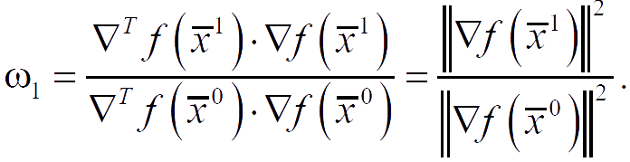
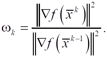
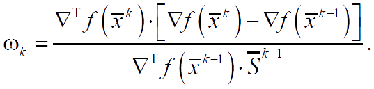
After n+1 iterations ( k = n), if the algorithm has not been stopped, the procedure is repeated cyclically with the replacement of x̅⁰ by x̅ⁿ⁺¹ and return to the first point of the algorithm. If the initial function is quadratic, then the (n+1)-th approximation will give the extremum point of this function. The described algorithm with plotting of ω_k using formulas corresponds to the Fletcher-Reeeves method of conjugate gradient.

In the modification of Polak-Ribier (Pshenichny’s), the method of conjugate gradients differs only by calculating:

In the case of quadratic functions, both modifications are approximately equivalent. In the case of arbitrary functions, nothing can be said in advance: somewhere one algorithm may be more effective, somewhere another.

Working with the "Optimizer" block

The vector of optimization criteria should be supplied to the input of the "Optimizer" block. Based on these values, using numerical optimization methods, the value of the output vector of optimization parameters is selected so that the values of the criteria are within the required range.

Input Ports

Parameter name	Description	Communication line type
in	Optimization criteria vector	Mathematical

Output Ports

Parameter	Description	Communication line type
out	Optimization parameter vector	Mathematical

Properties

Title	Parameter	Description	By default	Data type
Parameter Optimization Mode	optmode	Optimization is carried out either dynamically during one simulation cycle of the system, changing the optimization parameter directly during the simulation, or by the complete transient process of the system using a series of successive simulation cycles, in each of which the value of the optimized parameter is updated ("By the complete transient process", "In dynamics with stop", "In dynamics continuously")	In dynamics continuously	Enumeration
Duration of analysis step for optimization criteria when calculating in dynamics, sec	optstep	How often the criteria will be analyzed during the simulation and, consequently, the value of the optimized parameter will change. The option makes sense only when the dynamic parameter optimization mode is set	1	Real
Set initial point manually	manualpoint	Checkbox that allows you to set the starting point manually	None	Binary
Initial approximation of block outputs	x0	Initial values of optimized parameters from which the calculation begins	[1]	Array
Minimum values of block outputs	ymin	Shows the minimum values that can take the optimized parameters	[0]	Array
Maximum values of block outputs	ymax	Shows the maximum values that can take the optimized parameters	[10]	Array
Absolute error of selection of output values	yabserror	Minimum step at which output values can be varied	[0.001]	Array
Initial output increment	dparams	The magnitude of the change in the values of the outputs at the first selection step	[]	Array
Minimum values of input optimization criteria	umin	Lower limit of the target range of optimization criteria. Set as a linear array if there are more than one criteria	[0]	Array
Maximum values of input optimization criteria	umax	The upper limit of the target range of the optimization criteria. Set as a linear array if there are more than one criteria	[0.02]	Array
Type of total optimization criterion	usumtype	Method of criteria folding for the formation of the goal function ("Additive", "Quadratic", "Minimax", "Multiplicative")	Additive	Enumeration
Method of optimization	optmethod	Numerical optimization method used ("Search-2", "Search-4", "Simplex", "Method of the fastest descent", "Method of conjugate gradients")	Simplex	Enumeration
Maximum number of repetitive simulations in the calculation by the complete transient process	maxiter	The maximum number of repeated simulations during which the algorithm will try to select the optimal parameters. If at the end of the specified number of calculations, the values of the parameters that meet the optimization criteria were not found, then the calculation is interrupted. The option is only applicable if the optimization mode “By the complete transient process” is selected	500	Integer
Output of information about the optimization process	printoptinfo	Enabling the option means issuing information messages about the value of parameters and optimization criteria after each change in the system calculation process	None	Binary

Parameters

The block has no parameters.

Examples

Examples of block application: